Image Gallery
|
|
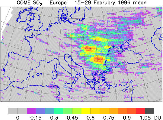
| Figure 1: GOME SO2 total columns above Europe averaged over the period 15-29 February 1996. Enhanced SO2 levels observed in Eastern Europe are most likely emissions from coal power plants. During this period surface temperatures were extremely low so that private household may also have contributed to the high SO2 values (Eisinger and Burrows, 1999) |
|
|
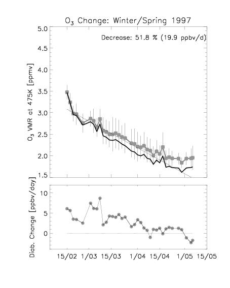
| Figure 2: GOME time series of mean Arctic vortex ozone volume mixing ratios on the 475 K isentropic potential temperature surface (about 19 km altitude) during Arctic winter/spring season 1996/97. Solid points are the GOME results and error bars are the 1sigma standard deviations from averaging inside the polar vortex. The solid line represents the ozone time series, where the subsidence of the vortex has been calculated from diabatic heating rates and the accumulated diabatic ozone changes (bottom plot) were subtracted from the original times series. This curve provides an estimate of the true chemical ozone loss during the course of the winter. Between middle of February and early May 1997 an accumulated ozone loss of 52% have been derived (Bramstedt et al. 2000). For more information on ozone profile retrieval contact Kai-Uwe Eichmann. |
|
|
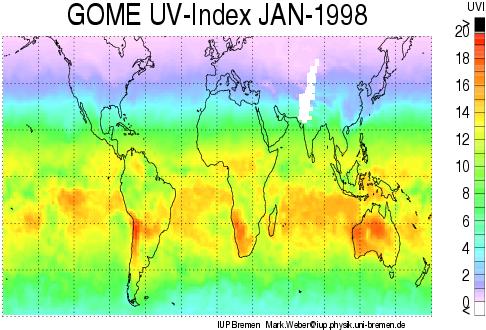
| Figure 3: Mean surface UV index in January 1998 derived from GOME data. Radiative transfer calculations using the total ozone information from GOME determines the clear-sky surface UV flux. Cloud information are derived from estimation of the Lambertian equivalent reflectivitity (LER), which is defined as the surface albedo in an aerosol and cloud free atmosphere that provides the appropiate top-of-atmosphere radiance observed by GOME. High LER are indicative of the presence of clouds and the LER values are used to estimate the cloud attenuation of the UV surface flux. The UV index is an erythemally weighted integrated surface flux (Erythema=sun burn) and is normally calculated for local noon time (maximum exposure) condition. |
|
|
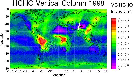
| Figure 4: Formaldehyde annual mean vertical columns from GOME in 1998. High amounts of HCHO have been observed in particular above rain forests in equatorial regions. They are probably due to high biogenic emissions of terpenes and isoprenes. Further information about HCHO evaluation is available on the IUP DOAS page) or please contact Folkard Wittrock. |
|
|
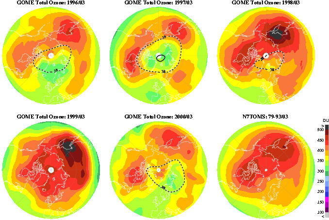
| Figure 5: March northern hemispheric total ozone distributions 1996-2000 (from left to right and top to bottom) and climatogical mean from Nimbus7/TOMS 1979-1993 (bottom right). After extended periods of very low stratospheric temperatures in the polar region during winter, low total ozone columns were observed in March (1996, 1997, and 2000). The mean position of the polar vortex, a stratospheric cyclone, where low ozone was measured is indicated by the dashed contour. High total ozone values throughout the northern hemisphere (NH) were found following winters with warmer stratospheric temperatures (1998 and 1999). The Arctic stratospheric winter/spring seasons exhibit high interannual dynamic variability in meteorology and ozone and leads to very different levels of chemical ozone depletion each year. The Greenwich meridian (0ºE) points towards the bottom in the stereographic projection. |
Author:
M. Weber
Last change: 12/21/2000
Institute of Environmental
Physics, University of Bremen