

Bild des Monats
Juni 2026:

Menschliche Aktivitäten treiben Afrika in Richtung Dürre
Afrika erwärmt sich schneller als je zuvor. Dürren werden häufiger, Ernten scheitern, Wasserquellen versiegen. Aber wie viel davon ist wirklich vom Menschen verursacht? Eine neue Studie gibt Antworten speziell für den afrikanischen Kontinent.
Ein internationales Team unter Mitwirkung von Wissenschaftlern des IUP nutzte Klimabeobachtungen sowie Klimamodelldaten um mit einer spezifischen Methode menschliche von natürlichen Einflüssen zu trennen.
Die Haupttreiber der Erwärmung in Afrika sind Treibhausgase (CO₂, Methan) und Landnutzungsänderungen. Gesamterwärmung durch Menschen liegt bei etwa +0.8°C über vorindustriellem Niveau. Dies geht einher mit starkem Temperaturanstieg und deutlich trockeneren Bedingungen. Eine wichtige Erkenntnis: Landnutzung wird unterschätzt. Unabhängig von den betrachteten Klimaszenarios wird Afrika voraussichtlich mehr Dürren, zunehmende Hitzewellen, und geringere Ernten zu beklagen haben. Dies ist von besonderer Bedeutung, da viele Länder Afrikas stark abhängig von der Landwirtschaft sind und über geringe Wasserressourcen sowie geringere finanzielle Mittel zur Klimaanpassung verfügen.
Referenz:
Swain, B., Vountas, M., Song, R. et al. Human-induced temperature rise is driving Africa towards drought-prone climatic conditions. Sci Rep 16, 630 (2026). https://doi.org/10.1038/s41598-025-34010-6
Mai 2026:

Das stratosphärische Ozon spielt eine entscheidende Rolle beim Schutz des Lebens auf der Erde vor schädlicher ultravioletter Strahlung, was die Bedeutung einer kontinuierlichen Überwachung des Ozongehalts unterstreicht. Aus diesem Grund sind zuverlässige Trendschätzungen aus mehreren zusammengeführten Langzeit-Ozondatensätzen (a bis f) hilfreich, um diese Veränderungen zu verstehen und zu überprüfen.
Jedes Feld der Abbildung zeigt Ozon-Trends aus einem anderen zusammengeführten Limb-Profil-Datensatz, basierend auf Kombinationen mehrerer Satelliteninstrumente: GOZCARDS (a), SAGE-CCI-OMPS (b), SAGE-OSIRIS-OMPS (c), SAGE-SCIA-OMPS (d), SAGEII-OSIRIS-SAGEIII (e) und SWOOSH (f).
Wir analysieren den Zeitraum von 2000 bis 2024, um die Erholung der Ozonschicht in der Stratosphäre zu untersuchen, und vergleichen dabei die Ergebnisse der einzelnen Datensätze. In der oberen Stratosphäre zeigen die verschiedenen zusammengeführten Datensätze sehr ähnliche positive Trends, was auf eine eindeutige Erholung in diesen Höhen hinweist. Oberhalb der Tropopause (gestrichelte Linie) werden in den Tropen negative Trends beobachtet. Die schraffierten Bereiche kennzeichnen Regionen ohne statistische Signifikanz (2σ) und treten häufiger in den Tropen und in der Nähe der Tropopause auf.
Während die stärksten positiven Trends in der oberen Stratosphäre auftreten, befindet sich ein großer Teil des gesamten atmosphärischen Ozons in der unteren Stratosphäre, wodurch Trends in dieser Region für Veränderungen der gesamten Ozonsäule besonders relevant sind. Unsere Analyse vergleicht die Trends der gesamten Ozonsäule mit den Trends der stratosphärischen Säule und zeigt eine enge Übereinstimmung, was darauf hindeutet, dass langfristige Veränderungen des gesamten Ozons in erster Linie durch die Variabilität des stratosphärischen Ozons bestimmt werden, wobei die Troposphäre nur einen geringen Beitrag leistet.
Literatur
Auffarth, B., Weber, M., Rozanov, A., Arosio, C., Burrows, J. P., Coldewey-Egbers, M., Davis, S. M., Degenstein, D., Dubé, K., Frith, S. M., Froidevaux, L., Loyola, D., Fioletov, V. E., Sofieva, V., van der A, R., and Wild, J. D.: Consistency Between Zonal Mean Stratospheric and Total Column Ozone Trends (2000–2024), EGUsphere [preprint], https://doi.org/10.5194/egusphere-2026-2576, 2026.
April 2026:

Viele Meereismodelle stützen sich auf sehr einfache Darstellungen der Meereisalbedo und nutzen diese als Einstellparameter, wobei sie Genauigkeit oder komplexere physikalische Modelle zugunsten von Einfachheit und geringeren Rechenaufwand opfern. Hier stellen wir einen neuartigen datengesteuerten Rahmen vor, um eine analytische Formulierung für die Albedo des Meereises (Atmojo et al., 2025) mithilfe von PySR, einem Python-Paket für symbolische Regression (Cranmer et al., 2020), zu ermitteln, mit dem Ziel, bestehende Parametrisierungen der Meereis-Albedo zu verbessern. Zum Trainieren unserer Machine-Learning-Modelle verwenden wir Satellitenbeobachtungen und Reanalyseprodukte, die tägliche, mehrjährige panarktische Daten mit einer räumlichen Auflösung von 25 km liefern. Der Kern unserer Methodik, dargestellt in der oberen Abbildung, ist die Parsimonie (Beucler et al., 2025): Wir entwickeln ein Modell, das die beobachtete Albedo des Meereises mit möglichst geringer Komplexität ausreichend gut reproduziert und somit die Einfachheit und Interpretierbarkeit stärkt.
Die untere Abbildung zeigt, dass die in unserer Studie vorgeschlagene Gleichung den beobachteten saisonalen Zyklus im Vergleich zur Parametrisierung von Parkinson und Washington (1979) (PW79) gut wiedergibt. Im September zeigt die Referenzbeobachtung VIIRS einen Rückgang der Meereisalbedo, was im Widerspruch zum erwarteten Einfrierverhalten des arktischen Meereises steht, das durch den zunehmenden Sonnenzenitwinkel bedingt ist, der die Qualität und Genauigkeit des VIIRS-Albedo-Produkts beeinträchtigt. Wahrscheinlich aufgrund der spärlichen Beobachtungsdaten, die für September infolge der geringeren Sonneneinstrahlung verfügbar sind, stützt sich PySR stärker auf die vollständigen Daten aus den vorangegangenen Frühlings- und Sommermonaten. Folglich korrigiert unsere vorgeschlagene Gleichung potenzielle Messartefakte in den Septemberdaten effektiv, indem sie funktionale Beziehungen nutzt, die aus Monaten mit besserer Erfassung gelernt wurden.
Referenzen:
Atmojo, D. W., Weigel, K., Grundner, A., Holland, M. M., Sidorenko, D., and Eyring, V.: Data-driven equation discovery of a sea ice albedo parametrisation, EGUsphere [preprint], https://doi.org/10.5194/egusphere-2025-3556, 2025.
Beucler, T., Grundner, A., Shamekh, S., Ukkonen, P., Chantry, M., Lagerquist, R.: Distilling Machine Learning’s Added Value: Pareto Fronts in Atmospheric Applications, Artificial Intelligence for the Earth Systems, https://doi.org/10.1175/AIES-D-24-0078.1, 2025.
Cranmer, M., Sanchez-Gonzalez, A., Battaglia, P., Xu, R., Cranmer, K., Spergel, D., and Ho, S.: Discovering Symbolic Models from Deep Learning with Inductive Biases, https://doi.org/10.48550/ARXIV.2006.11287, publisher: arXiv Version Number: 2, 2020.
März 2026:

Die IUP-Ozeanographen Oliver Huhn, Jolanda Grimm und Andreas Rogge befinden sich derzeit an Bord des Forschungs-Eisbrechers „Polarstern“, um an der „Summer Weddell Outflow Study“ (SWOS) teilzunehmen. Durch die Entnahme von Wasserproben und die Erfassung von Unterwassersensordaten untersuchen sie die Rolle der Wassermasseumwandlung und -zirkulation für die Kohlenstoffbilanz des westlichen Weddellmeers.
Februar 2026:

Oben links: Korrelation zwischen der effektiven (Anti-)Zyklonstärke aus ERA5-Daten und der effektiven Ozonänderungsstärke, abgeleitet aus den Messungen der gesamten Ozonsäule durch Sentinel-5P. Es sind alle Zyklone (blau) und Antizyklone (rot) mit vollständiger S5P-Abdeckung zwischen 2019 und 2022 berücksichtigt.
Oben rechts: Beispiel einer Kollokation, das die Methode zur Ableitung der effektiven Zyklon- und Ozonänderungsstärke veranschaulicht. Dargestellt sind ein Zyklon in der oberen Troposphäre, definiert durch die Anomalie der geopotentiellen Höhe bei 250 hPa (untere Fläche) aus ERA5-Daten, und die kollokierte Gesamt-Ozonsäule, gemessen von S5P (obere Fläche). Die effektive Stärke sowohl des Zyklons als auch der damit verbundenen Ozonveränderung wird durch das Volumen quantifiziert, das zwischen der beobachteten Oberfläche und einer Referenzoberfläche eingeschlossen ist, die durch den Mittelwert an der Systemgrenze definiert ist. Dieses Volumen repräsentiert den Nettoanstieg des Ozons und den Nettoabfall des Drucks innerhalb des Zyklons im Verhältnis zu seiner Umgebung.
Unten links: Die geopotenzielle Höhe bei 250 hPa aus ERA5-Daten, die der unteren Fläche in der oben gezeigten Darstellung entspricht. Der Rand des Zyklons ist rot markiert, und der Sentinel-5P-Erfassungsbereich für den entsprechenden Überflug ist violett dargestellt.
Unten rechts: Die von Sentinel-5P gemessene Gesamt-Ozonsäule für denselben Überflug und denselben Zyklon, entsprechend der oberen Fläche in der oben gezeigten Darstellung.
Zyklone und Antizyklone stehen in Zusammenhang mit systematischen Schwankungen der gesamten Ozonsäule – ein Zusammenhang, der bereits zu Beginn des 20. Jahrhunderts erkannt wurde. Hier zeigen wir erstmals, dass satellitengestützte Messungen der gesamten Ozonsäule zur quantitativen Bewertung der Stärke synoptischer Ereignisse herangezogen werden können. Zu diesem Zweck führen wir Methoden ein, um die effektive Stärke der (Anti-)Zyklone aus ERA5-Daten und der aus Sentinel-5P-Messungen abgeleiteten Ozonänderung zu berechnen, die für Nadir-Beobachtungen optimiert sind, wobei die hohe horizontale Auflösung berücksichtigt und die Ozonanomalie aller Pixel innerhalb des (Anti-)Zyklonbereichs einbezogen wird. Die Anwendung dieses Ansatzes auf alle vollständig erfassten Zyklone und Antizyklone zwischen 2019 und 2022 zeigt eine starke Korrelation zwischen der Stärke synoptischer Ereignisse und der Stärke der induzierten Ozonveränderung.
Diese Beziehung zeigt, dass Messungen der gesamten Ozonsäule am Nadir dynamisch relevante Informationen über die Stärke von Systemen auf synoptischer Skala enthalten, und unterstreicht das Potenzial von Satelliten-Ozonbeobachtungen als wertvolle Eingangsgröße für die Datenassimilation sowie für die Verbesserung der Darstellung und der Stärkeeinschätzung von Zyklonen und Antizyklonen in numerischen Wettervorhersagemodellen.
Januar 2026:

Wissenschaftler am Institut für Umweltphysik sind auf die Entwicklung, den Einsatz und die Anwendung verschiedener Sensortypen spezialisiert, um Emissionen anthropogener Treibhausgase durch die Messung der Verteilung von Methan (CH₄) und Kohlendioxid (CO₂) in der Atmosphäre zu lokalisieren und zu quantifizieren. Um die Emissionen anhand dieser Verteilungen genau abschätzen zu können, sind präzise Daten zu den Konzentrationen und den lokalen Windfeldern erforderlich. Da viele wichtige Emissionsquellen Treibhausgase in Bodennähe ausstoßen, ist es wichtig, die relevanten Daten in Bodennähe zu erfassen. Dies kann mit einem mobilen Labor erreicht werden. Im Jahr 2025 gelang es dem Team, einen Windsensor, einen In-situ-Spurengasanalysator und ein nach oben gerichtetes Spektrometer zur Messung der Treibhausgas-Säulenkonzentration in den mobilen Labor-Lkw des IUP zu integrieren.
Erste Testfahrten wurden im Nordwesten Deutschlands durchgeführt, in Regionen, in denen Quellen für biogenes (Landwirtschaft) und geogenes (z. B. Gasanlagen) Methan in der Nähe liegen. Ein Beispiel ist in der obigen Abbildung dargestellt. Die gleichzeitige Messung von Methan und Ethan ermöglicht eine klare Unterscheidung zwischen biogenem und geogenem Methan, da nur Letzteres Ethan mitemittiert. Die Messungen der Treibhausgaskonzentrationen und Windfelder durch das mobile Labor ergänzen eine ähnliche Sensoraufstellung an einem Motorsegler (Bild des Monats Juni 2022). Es werden kombinierte Daten aus der Luft und dem mobilen Labor gesammelt, um zu untersuchen, wie der kombinierte Datensatz dazu beitragen kann, die unabhängige Emissionsquantifizierung zu verbessern. Studierende, die daran interessiert sind, mit uns zusammenzuarbeiten, sind jederzeit willkommen, insbesondere wenn sie einen Führerschein für Lkw (C1/C) besitzen.
Kontakt:
Heinrich Bovensmann: heinrich.bovensmann@uni-bremen.de
Jakob Thoböll: jthoboell@iup.physik.uni-bremen.de
Dezember 2025:

Oben: Schematische Darstellung der Auswirkungen meteorologischer Veränderungen und Emissionsveränderungen auf die dreijährigen Schwankungen der PM2,5-Belastung
im Perlflussdelta
Unten: Beiträge lokaler Emissionen (Emis_L), externer Emissionen (Emis_O) und meteorologischer Faktoren (Meteo) zu den Veränderungen der PM2,5-Konzentrationen
Konzentrationen (fett gedruckt; Anstiege rot, Rückgänge blau) und regionale Quellenbeiträge im Perlflussdelta während der kalten Jahreszeiten 2015–2017, abgeleitet aus den WRF-CMAQ-Simulationen (Details siehe Qu et al., 2025)
Anhaltende PM2,5-Belastung im Perlflussdelta (2015–2017): Meteorologie vs. Emissionsreduktionen
Feinstaub (PM2,5) stellt eine ernsthafte Gefahr für die menschliche Gesundheit dar, weshalb Maßnahmen zur Minderung der regionalen PM2,5-Belastung erforderlich sind. In China, einem der am stärksten von schwerer PM2,5-Belastung betroffenen Länder, haben Emissionskontrollmaßnahmen oft zu einer wirksamen Senkung der PM2,5-Werte geführt. Allerdings darf die Rolle der Meteorologie bei der Entstehung mehrjähriger Schwankungen der PM2,5-Belastung nicht übersehen werden. In dieser Studie untersuchten wir die PM2,5-Veränderungen in der Pearl River Delta-Region in Südchina während der kalten Jahreszeiten 2015-2017, einem Zeitraum, in dem die PM2,5-Belastung trotz rascher Emissionsreduktionen anhielt.
Wir haben festgestellt, dass die anhaltende PM2,5-Belastung während dieser drei kalten Jahreszeiten in engem Zusammenhang mit den Veränderungen der meteorologischen Bedingungen stand, die mit dem Übergang von El Niño im Jahr 2015 zu La Niña im Jahr 2017 einhergingen. Dieser Übergang führte zu stärkeren Nordwinden, wodurch der regionenübergreifende Transport von PM2,5 und seinen Vorläufern aus stärker verschmutzten Regionen in Nord- und Zentralchina verstärkt wurde, während gleichzeitig die lokale PM2,5-Produktion und -Anreicherung abgeschwächt wurde. Simulationen mit dem WRF/CMAQ-Modell zeigen außerdem, dass die PM2,5-Konzentrationen in den ersten beiden kalten Jahreszeiten zurückgingen und danach wieder anstiegen, wobei der Beitrag des regionalen Transports zu PM2,5 jedoch kontinuierlich zunahm, und zwar von 70 % im Jahr 2015 auf 74 % im Jahr 2016 und 78 % im Jahr 2017. Die entsprechenden Ergebnisse wurden in Atmospheric Chemistry and Physics (Qu et al., 2025) veröffentlicht.
Danksagung:
Diese Arbeit wird unterstützt durch das Nationale Schlüsselforschungs- und Entwicklungsprogramm Chinas, die Deutsche Forschungsgemeinschaft (DFG) im Rahmen der Exzellenzstrategie Deutschlands und das kofinanzierte DFG-NSFC-Projekt „Sino-German Air-Changes”.
Referenz:
Qu, K., Wang, X., Yan, Y., Jin, X., He, L.-Y., Huang, X.-F., Cai, X., Shen, J., Peng, Z., Xiao, T., Vrekoussis, M., Kanakidou, M., Brasseur, G. P., Daskalakis, N., Zeng, L. und Zhang, Y.: Unexpectedly persistent PM2.5 pollution in the Pearl River Delta, South China, in the 2015–2017 cold seasons: the dominant role of meteorological changes during the El Niño-to-La Niña transition over emission reduction, Atmos. Chem. Phys., 25, 16983–17007, https://doi.org/10.5194/acp-25-16983-2025, 2025.
Kontakt:
Kun Qu (qukun@uni-bremen.de)
November 2025:
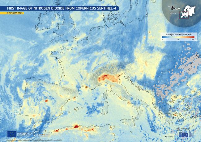
Am 8. Oktober führte das europäische Instrument Sentinel-4 seine ersten atmosphärischen Messungen durch. Dieses Instrument befindet sich in einer geostationären Umlaufbahn und wird stündlich Daten zu Stoffen wie Ozon, NO2, Formaldehyd, SO2 und Glyoxal sowie zu Wolken und Aerosolen über Europa liefern. Die Prozessoren für NO2 und Glyoxal wurden am Institut für Umweltphysik der Universität Bremen entwickelt, und das Team ist derzeit damit beschäftigt, die Daten auszuwerten und die Algorithmen zu optimieren.
Das Sentinel-4-Instrument ist das letzte einer Konstellation von drei geostationären Instrumenten, die die Zusammensetzung der Atmosphäre über Asien (GEMS), Nordamerika (TEMPO) und nun auch Europa (Sentinel-4) beobachten. Es geht auf die ersten Vorschläge für ein geostationäres Instrument namens GEOSCIA zurück, die Prof. John Burrows und seine Kollegen vor mehr als 20 Jahren vorgelegt hatten.
Copernicus News: https://www.copernicus.eu/en/media/image-day-gallery/first-image-nitrogen-dioxide-copernicus-sentinel-4
ESA news: https://www.esa.int/Applications/Observing_the_Earth/Copernicus/Sentinel-4/Sentinel-4_offers_first_glimpses_of_air_pollutants
Oktober 2025:
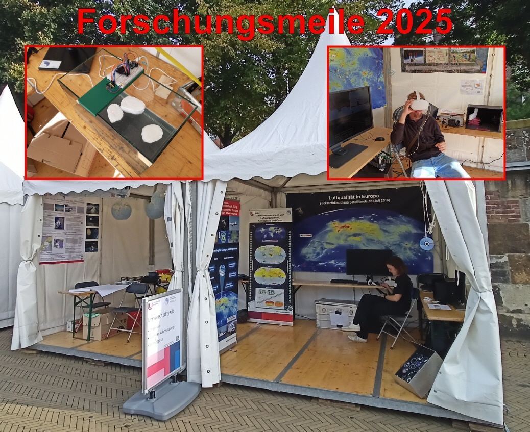
Das IUP bei der Forschungsmeile 2025
Auch dieses Jahr nahm das IUP wieder an der Forschungsmeile im Rahmen der Maritimen Woche an der Weserpromenade „Schlachte“ teil. Die Abteilungen Fernerkundung und Physik und Chemie der Atmosphäre präsentierten am 20. und 21. September dem Publikum Messmethoden und Forschungsergebnisse aus den Themenbereichen Meereis, Luftverschmutzung und Klimawandel. Außerdem konnten die Besucher eine virtuelle Reise in einem Stratosphärenballon antreten (siehe auch „Bild des Monats“ August 2025).
Kontakt: Stefan Noël (stefan.noel@iup.physik.uni-bremen.de)
September 2025:
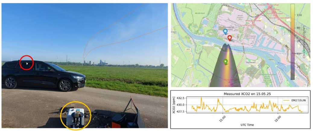
Beobachtung von CO₂ aus dem Bremer Stahlwerk
Das Bild zeigt eine Messkampagne nahe der Bremer Stahlfabrik – einem der größten CO₂-Emittenten der Stadt – im Frühjahr 2025. Um besser zu verstehen, wie viel CO₂ freigesetzt wird, setzte das Team der Abteilung für Nah-IR-Fernerkundung und In-situ-Messungen des IUP eine Reihe von mobilen Instrumenten rund um das Gelände ein.
Gase wie CO₂, CO und NO₂ wurden direkt in der Luft in der Nähe des Werks mit einer Kombination aus In-situ-Analysatoren, einem DOAS-Gerät (roter Kreis) und zwei EM27/SUN-FTIR-Solarabsorptionsspektrometern gemessen (orangener Kreis und Daten).
Zur Interpretation der Daten verwendet das Team Gaußsche Plume-Modelle, um zu simulieren, wie sich die Emissionen unter verschiedenen Wind- und Wetterbedingungen in der Atmosphäre ausbreiten.
Ziel des Projekts ist es, die Überwachung von Emissionen aus großen industriellen Quellen zu verbessern und eine genauere, wissenschaftlich fundierte Klimaberichterstattung zu unterstützen, beginnend hier in Bremen.
August 2025:
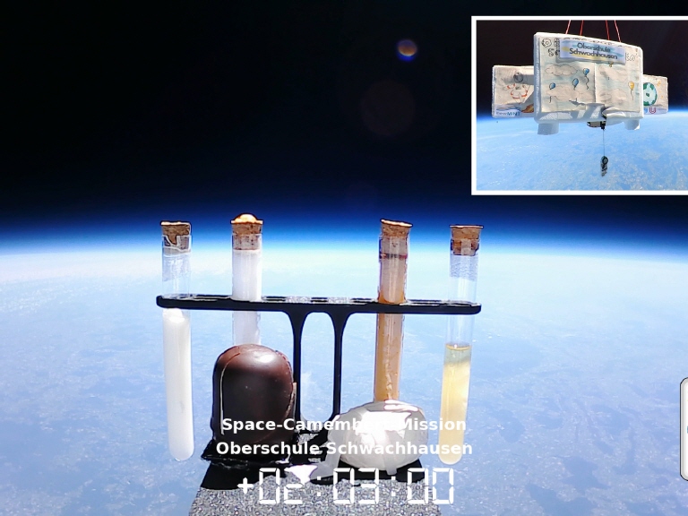
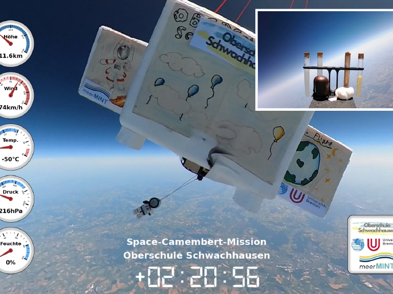

Am 20.06.2025 fand die Space-Camembert-Mission des Jugend forscht-Ateliers der neu gegründeten Oberschule Schwachhausen statt. Für diese Mission wurde gemeinsam mit den Schüler:innen eine Stratosphärensonde gebaut, die mithilfe eines Wetterballons bis in eine Höhe von fast 40 Kilometern aufstieg. Dabei wurden zahlreiche meteorologische Parameter gemessen und Experimente durchgeführt.
Am höchsten Punkt ihres Fluges hatte die Sonde etwa 99,5% der Erdatmosphäre unter sich gelassen und die Aufnahmen der Kameras vermitteln eindrucksvoll, warum viele Astronaut:innen nach ihrer Rückkehr aus dem All berichteten, dass ihnen die Atmosphäre sehr dünn und verletzlich vorkam. Die Idee zur Mission entstand am Institut für Umweltphysik der Universität Bremen, das zusammen mit dem meerMINT Projekt, der Senatorin für Kinder und Bildung Bremen und dem Deutschen Zentrum für Luft- und Raumfahrt die Mission maßgeblich unterstützt hat.
Die Highlights im 9-Minuten-Video: https://youtu.be/o9FdLZvttq4
Die Highlights im 5-Minuten-360°-Video: https://youtu.be/EIvRPPxC4kE
Zusammenfassung und Interviews im 4-Mintuen-Video: https://youtu.be/9JP0iYdbI40
Juli 2025:
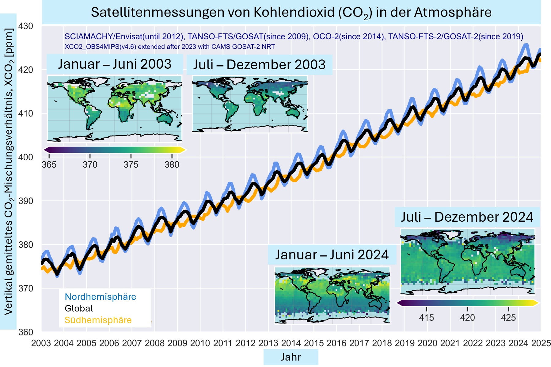
Zeitserien und globale Karten des atmosphärischen CO2-Mischungsverhältnisses. Wie man sieht, steigen die atmosphärischen CO2-Konzentrationen ungebremst weiter an, trotz weltweiter Bemühungen, CO2-Emissionen zu reduzieren. Die Daten wurden vom IUP der Universität Bremen durch Kombination der Messungen verschiedener Satelliten erstellt und vom Copernicus Klimawandel-Dienst (https://climate.copernicus.eu/) für einen kürzlich erschienenen Bericht verwendet (siehe European State of the Climate (ESOTC) 2024, https://climate.copernicus.eu/esotc/2024).
Juni 2025:
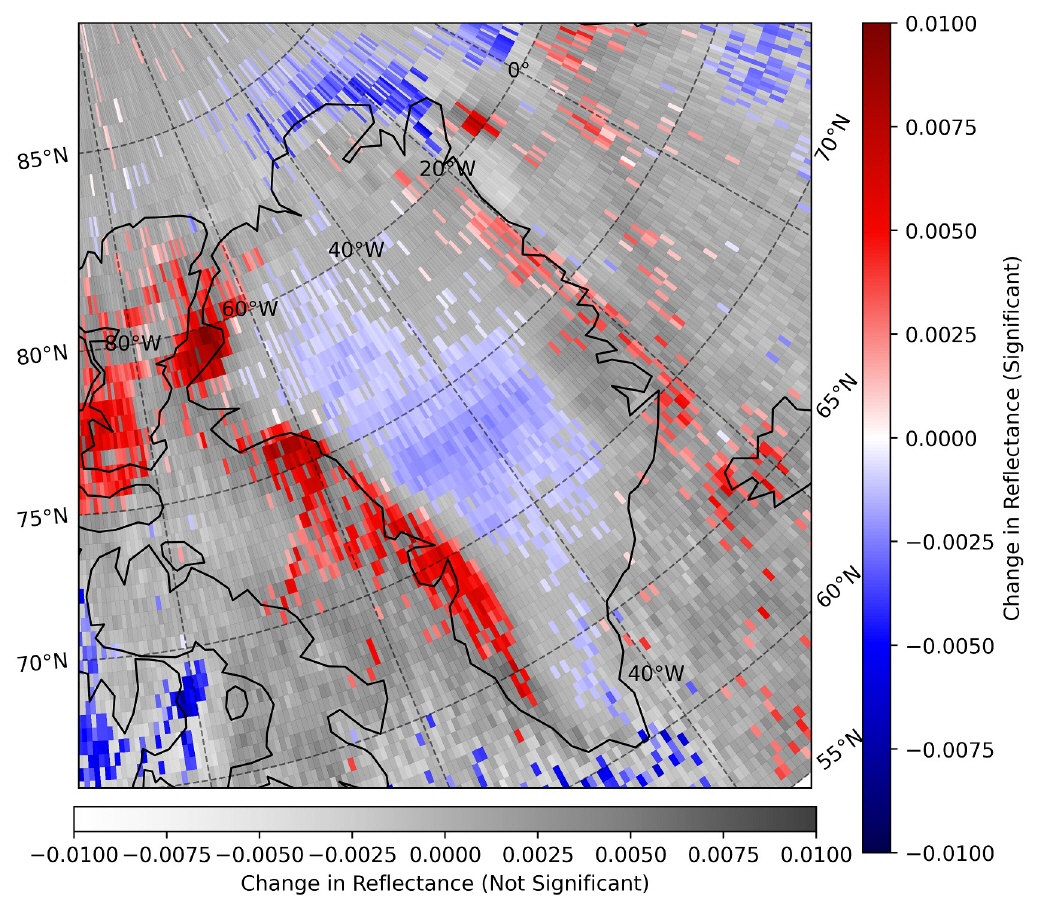
Studien zur Veränderungen des von Grönland reflektierten Sonnenlichts zwischen 2007 und 2024
Die zugrundeliegenden Daten wurden von einem Satelliteninstrument (GOME-2) gemessen. Dabei handelt es sich um ein die Erdoberfläche und Erdatmosphäre abtastendes Spektrometer, dass in der Lage ist, das reflektierte Sonnenlicht bei verschiedenen Wellenlängen zu messen (die verschiedenen Farben im sichtbaren Spektrum des Sonnenlichts entsprechen).
Das Bild zeigt farbige Bereiche (blau bis rot) an denen die Veränderungen über den Zeitraum von 17 Jahren (statistisch gesehen) aussagekräftig und zuverlässig sind, während graue Bereiche zeigen, wo die Veränderungen nicht stark genug sind, um sicher zu sein. Wichtig ist, dass blaue Bereiche, wie im Zentrum Grönlands, zeigen, wo das reflektierte Sonnenlicht zwischen 2007 und 2024 abgenommen hat, und rote Bereiche, wie z.B. die Westküste Grönlands, zeigen, wo es stattdessen zugenommen hat. Derzeit beschäftigt sich das Team mit den möglichen Ursachen solcher Veränderungen.
Mai 2025:

Schwankungen des Ozons in der unteren Stratosphäre (10-20 km Höhe) sind mit Wetterphänomenen in der Troposphäre verbunden, wie in dieser Abbildung beispielhaft dargestellt. Hier ist das Ozon in 10 km Höhe (oberes Feld) über einem Wirbelsturm in der mittleren Troposphäre (7,5 km Höhe, unteres Feld) erhöht.
In einer Studie von Monsees et al. (2024) wurden die Auswirkungen troposphärischer Wirbelstürme auf das Ozon in der unteren Stratosphäre anhand von Limb- Messungen durch Satelliten, hier OMPS-LP, untersucht. Da die meteorologischen Daten, die als Input für numerische Wettervorhersagen benötigt werden, in der arktischen Region recht spärlich sind, kann das Potenzial der Verwendung von Ozon in der unteren Stratosphäre für die Assimilation in Wettermodelle für die Verbesserung der Wettervorhersagen in dieser Region von Bedeutung sein.
Das obere Feld zeigt in Farbe das OMPS-LP-Ozon in Abhängigkeit von der Satellitenbahnposition (Datenpunktnummer) und der Höhe. Die farbigen Linien stellen Niveaus mit konstanten Ozonwerten von 80, 150 bzw. 250 ppb dar. Das Absinken dieser Linien in der Höhe, insbesondere bei 250 ppb, korreliert gut mit dem Luftdruckabfall innerhalb des Wirbelsturms und kann als Indikator für die Aktivität des troposphärischen Wirbelsturms verwendet werden.
Referenz: Monsees, F., Rozanov, A., Burrows, J. P., Weber, M., Rinke, A., Jaiser, R., and von der Gathen, P.: Relations between cyclones and ozone changes in the Arctic using data from satellite instruments and the MOSAiC ship campaign, Atmos. Chem. Phys., 24, 9085–9099, https://doi.org/10.5194/acp-24-9085-2024, 2024.
April 2025:
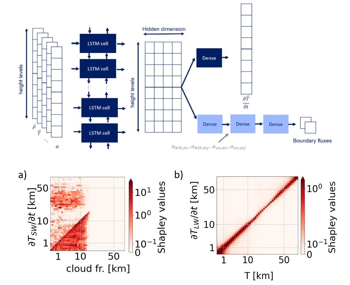
Um die künftigen Auswirkungen des Klimawandels abzuschätzen, stützen wir uns auf Klimaprojektionen, die von Erdsystemmodellen (ESM) erstellt werden. Die Strahlung spielt eine entscheidende Rolle bei der Steuerung des Klimasystems und gehört zu den rechenintensivsten Komponenten von ESMs.
Um Rechenressourcen zu sparen, werden Strahlungsberechnungen oft weniger häufig oder mit geringerer Detailgenauigkeit durchgeführt, was zu Unsicherheiten bei der Wechselwirkung zwischen Wolken und Strahlung führt.
Hier entwickeln wir ein Modell des maschinellen Lernens (ML), um die Strahlungsberechnungen zu beschleunigen und gleichzeitig die Genauigkeit zu erhalten. Konkret verwenden wir ein bidirektionales Langzeitgedächtnis (Bi-LSTM), das das vertikale Profil jeder Säule des Modells in Aufwärts- und Abwärtsrichtung abtastet.
Dies soll die Aufwärts- und Abwärtsflüsse nachahmen, die in der Strahlungsparametrisierung eines bekannten Klimamodells, dem nicht-hydrostatischen ICOsahedral-Modell (ICON), berechnet werden. Unser ML-basiertes Modell sagt zuverlässig die Erwärmungsraten sowohl für das Sonnenlicht (kurzwellige Strahlung) als auch für die Wärme von Erde und Atmosphäre (langwellige Strahlung) voraus. Wir analysieren die Vorhersagen des ML-basierten Emulators und zeigen, dass er die zugrunde liegenden physikalischen Zusammenhänge erfolgreich erfasst. Wir stellen fest, dass das ML-Modell lernt, dass Wolken eine entscheidende Rolle spielen. Abbildung a) zeigt, dass eine Wolke in einer Höhe von z. B. 10 km einen starken Einfluss auf die kurzwellige Temperaturtendenz auf derselben Höhe und auch auf jeder darunter liegenden Ebene hat, da die Wolke das einfallende Sonnenlicht absorbiert und reflektiert, was zu einer geringeren Erwärmung unterhalb der Wolke führt.
Die reflektierte Strahlung kann aber auch zu einer Erwärmung der Stratosphäre führen. Für die langwellige Strahlung hat das ML-Modell richtig erkannt, dass die Temperatur lokal wichtig ist, aber auch benachbarte Zellen beeinflusst, was durch die diffuse diagonale Linie in Abbildung b) angezeigt wird; dies ist physikalisch korrekt, da die Atmosphäre selbst eine Quelle langwelliger Strahlung ist und die Stärke durch die Temperatur bestimmt wird.
Katharina Hafner, Fernando Iglesias-Suarez, Sara Shamekh, et al. Interpretable Machine Learning-based Radiation Emulation for ICON. ESS Open Archive . November 15, 2024.
DOI: 10.22541/essoar.173169996.65100750/v1
https://essopenarchive.org/users/856312/articles/1240793-interpretable-machine-learning-based-radiation-emulation-for-icon
März 2025:
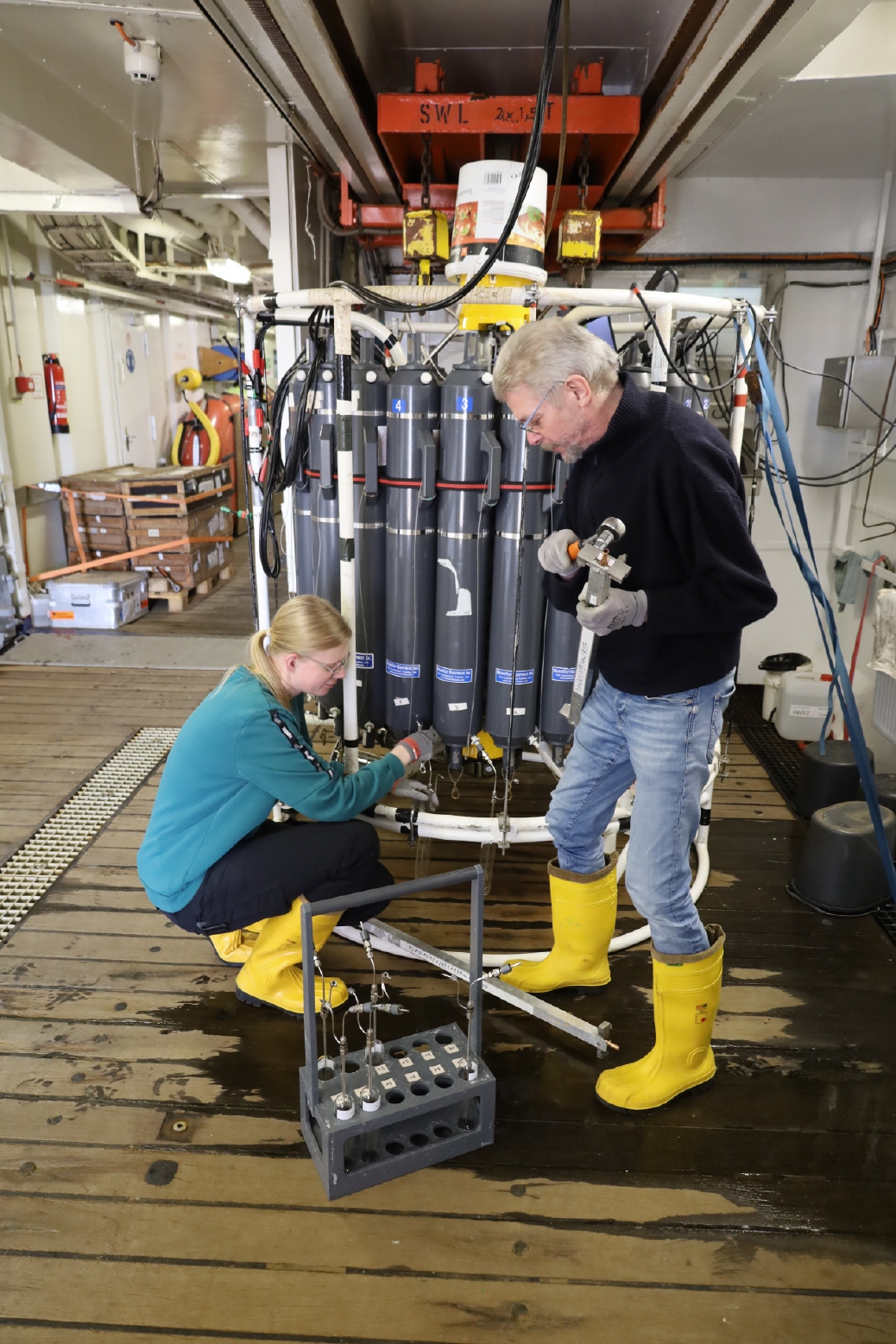
Lara Aschenbeck und Oliver Huhn vom Institut für Umweltphysik (IUP), Abteilung Ozeanographie, bei der Probennahme an Bord des Forschungseisbrechers Polarstern im Weddellmeer. Auf der Polarstern-Expedition PS146 (HAFOS/COSMUS-2) nehmen die beiden Meerwasserproben für die anthropogenen Spurengase FCKW und SF6 sowie die Edelgase Helium und Neon, die später am IUP gemessen und ausgewertet werden.
Die FCKW- und SF6-Messungen geben Aufschluss über die Zeitskalen des ozeanischen Transports und der Aufnahme von anthropogenem Kohlenstoff, während die Edelgase die Berechnung der Beiträge der geschmolzenen Gletscher ermöglichen. Foto: Martin Losch.
Februar 2025:
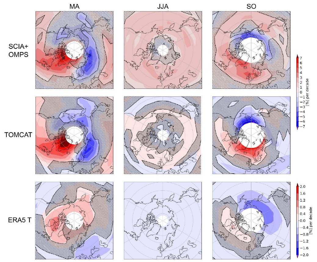
Asymmetrien in den Ozontrends in den nördlichen hohen Breiten wurden über den Zeitraum 2004-2022 mit Hilfe von Satellitenbeobachtungen (dem fusionierten SCIA+OMPS-Datensatz des IUP) und dem chemischen Transportmodell TOMCAT (in Zusammenarbeit mit der Universität Leeds) untersucht. Diese Abbildung zeigt die jahreszeitlichen Ozontrends für SCIA+OMPS (obere Reihe) und für eine TOMCAT-Simulation mit vollständiger Chemie (untere Reihe) in 32 km Höhe für Frühling (MA), Sommer (JJA) und Herbst (SO). Während des Sommers sind die Trendfelder über die geografische Länge recht homogen und zeigen signifikante positive Werte von etwa 1 % pro Jahrzehnt für SCIA+OMPS und nahe Null für TOMCAT. Im Gegensatz dazu wird im Frühjahr und Herbst ein asymmetrisches Muster festgestellt.
Die starke zonale Asymmetrie in den Frühjahrstrends von SCIA+OMPS wird von TOMCAT sehr gut erfasst, wobei sich das positive Maximum über dem Nordatlantiksektor befindet. Die negativen Werte zwischen Skandinavien und Sibirien sind ebenfalls statistisch signifikant (auf 2σ-Niveau), sowohl für die Beobachtungen als auch für das Modell. Ein ähnliches bipolares Muster findet sich auch in SO, allerdings stärker auf polare Breitengrade beschränkt und in der Länge verschoben. Dieses Muster wurde im Zusammenhang mit der Position des Polarwirbels und mit Trends in der potenziellen Wirbelstärke in der mittleren Stratosphäre weiter analysiert. Wir fanden heraus, dass Veränderungen der mittleren Polarwirbelposition und -stärke mit dieser Asymmetrie des Ozontrends zusammenhängen. Das Gesamtmuster unterlag in den letzten 40 Jahren dekadischen Veränderungen, wobei in den letzten beiden Jahrzehnten eine wahrscheinliche Verstärkung des Wirbels und eine Verschiebung in Richtung Nordamerika zu beobachten war.
Referenz
Arosio, C., Chipperfield, M. P., Rozanov, A., Weber, M., Dhomse, S., Feng, W., ... & Burrows, J. P. (2024). Investigating zonal asymmetries in stratospheric ozone trends from satellite limb observations and a chemical transport model. Journal of Geophysical Research: Atmospheres, 129(8), e2023JD040353.
Dezember 2024:
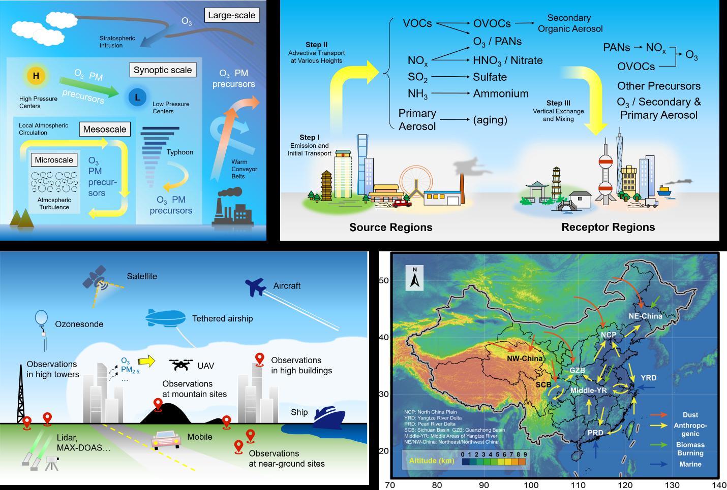
Der komplexe Einfluss des überregionalen Transports auf die Ozon- und Feinstaubbelastung und relative Ergebnisse in China
Der überregionale Transport (CRT) bezieht sich auf die weiträumige Bewegung von Schadstoffen über Entfernungen von zehn bis tausenden von Kilometern, die regionale Grenzen überschreiten und zur Luftverschmutzung in windabwärts gelegenen Gebieten beitragen. CRT ist von Natur aus komplex und wird von dynamischen Mechanismen angetrieben, die auf mehreren Ebenen wirken und von chemischen Umwandlungen während des Transports begleitet werden.
In dieser Studie wird speziell der Einfluss von CRT auf die Ozon- und Feinstaubbelastung in China untersucht, einem Land, das mit erheblichen Problemen bei der Luftqualität zu kämpfen hat. Ozon und Feinstaub stehen im Mittelpunkt dieser Analyse, da sie aufgrund ihrer mäßig langen Lebensdauer besonders anfällig für CRT sind. In dieser Übersicht (Qu et al., 2024) werden die jüngsten Erkenntnisse und Methoden zusammengefasst, wobei der Schwerpunkt auf der Verwendung von In-situ- und Fernerkundungsbeobachtungen sowie Modellierungsansätzen liegt, um die Beiträge von CRT zu quantifizieren und die beteiligten Prozesse im Detail zu untersuchen.
Unsere Analyse zeigt, dass die großen städtischen Cluster Chinas insgesamt stärker durch CRT als durch lokale Emissionen beeinflusst wurden. Darüber hinaus werden in der Studie die wichtigsten Transportwege und die entscheidenden dynamischen und chemischen Prozesse identifiziert, die die Luftverschmutzung in den verschiedenen Regionen des Landes beeinflussen (Abb. 1).
Danksagung:
Diese Arbeit wird vom National Key Research and Development Program of China, der Deutschen Forschungsgemeinschaft (DFG) im Rahmen der deutschen Exzellenzstrategie und dem kofinanzierten DFG-NSFC-Projekt Sino-German Air-Changes (448720203) unterstützt.
Referenz:
Qu, K., Yan, Y., Wang, X., Jin, X., Vrekoussis, M., Kanakidou, M., Brasseur, G.P., Lin, T., Xiao, T., Cai, X., Zeng, L., and Zhang, Y.: The effect of cross-regional transport on ozone and particulate matter pollution in China: A review of methodology and current knowledge, Sci. Total Environ., 947, 174196, https://doi.org/10.1016/j.scitotenv.2024.174196, 2024. Contact: Kun Qu (qukun@uni-bremen.de)
November 2024:
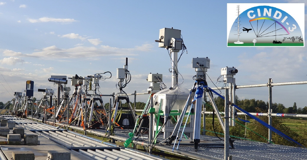
Im Mai und Juni 2024 fand in Cabauw, Niederlande, die dritte Cabauw INtercomparison of UV-Vis DOAS Instruments (CINDI-3) Kampagne statt. Mehr als 40 DOAS-Instrumente (Differential Optical Absorption Spectroscopy) von Forschungsgruppen aus der ganzen Welt kamen zusammen, um Messungen von Stickstoffdioxid (NO2) und vielen anderen Spurengasen durchzuführen. Eines der Ziele der Kampagne, die als halb-blinde Vergleichsmessungen organisiert war, bestand darin, die Konsistenz und Genauigkeit dieser Messungen zu ermitteln, die häufig zur Validierung von Satellitenbeobachtungen verwendet werden.
Als sekundäres Ziel wurde der Austausch von Informationen, Know-how und sogar Code zwischen den Gruppen durch tägliche Treffen und die Bildung mehrerer Arbeitsgruppen gefördert und erleichtert, die sich mit der Verbesserung spezifischer Aspekte der Abfrage befassten, wie z. B. der vertikalen Profilerstellung, der Anpassung von Glyoxal oder der Abfrage von Aerosolen.
Die DOAS-Gruppe der Universität Bremen nahm mit mehreren Instrumenten an der Kampagne teil, darunter ihr Standard-2d-MAX-DOAS-Instrument, das bildgebende Spektrometer IMPACT und ein mobiles DOAS, das von einem Auto aus betrieben wurde. Letzteres war Teil einer koordinierten Anstrengung zur Charakterisierung der NO2-Verteilung rund um den Kampagnenstandort mit mehreren Fahrzeugen, Ballons und Flugzeugüberführungen. Die Ergebnisse des Halbblindvergleichs und der verschiedenen Arbeitsgruppen werden in den kommenden Jahren veröffentlicht.
Oktober 2024:
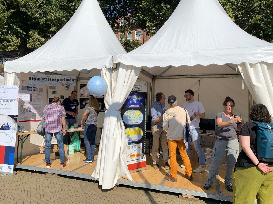
Am 21. und 22. September 2024 fand die diesjährige Forschungsmeile im Rahmen der Maritimen Woche an der Weserpromenade „Schlachte“ statt. Das IUP war diesmal mit einem Doppelzelt beteiligt, in dem die Abteilungen Fernerkundung, Physik und Chemie der Atmosphäre sowie Ozeanographie aktuelle Forschungsergebnisse präsentierten und mit dem Publikum interessante Diskussionen führten. Ein Highlight der Veranstaltung war eine Live-Schaltung zum Forschungsschiff „Polarstern“ im Nordpolarmeer.
Kontakt: Stefan Noël (stefan.noel@iup.physik.uni-bremen.de)
September 2024:
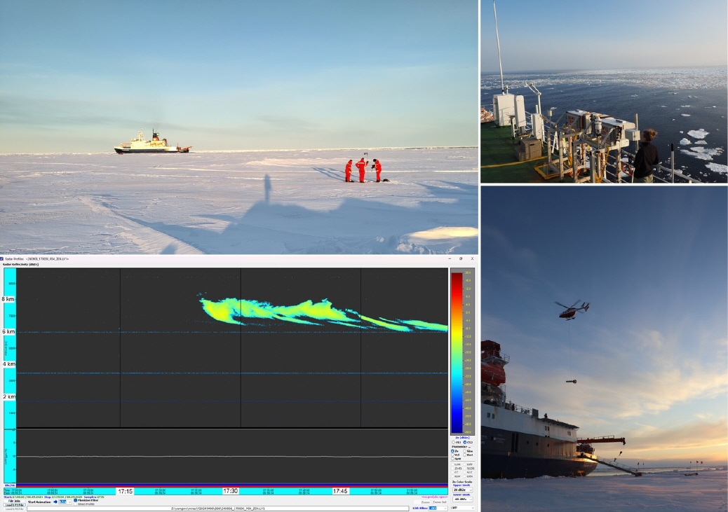
Zusammen mit der Universität zu Köln und dem AWI nimmt das IUP derzeit an der Fahrt PS144 ArcWatch2 der RV Polarstern teil. An Bord des Schiffes werden die Eigenschaften der Atmosphäre und des Meereises mit Mikrowellenradiometern und Radar (oben rechts) gemessen, um die numerische Wettervorhersage und die Satellitenbeobachtungen zu verbessern. Während der Eisstationen (oben links) werden die physikalischen Eigenschaften des Meereises und des Schnees im Detail gemessen: zum Beispiel die Größe der Schneekörner, die Eisdicke, der Salzgehalt und die Temperatur.
Diese Informationen werden benötigt, um die Mikrowellenmessungen auf dem Schiff und auch von den Satelliten aus zu interpretieren. Während der Eisstation beobachtete das aufwärtsgerichtete Wolkenradar Zirruswolken (unten links), die auch auf den Fotos unten rechts und oben links zu sehen sind. Um auch die Meereisdicke in größerem Maßstab zu beobachten, werden Hubschrauberflüge mit einem Instrument namens EM-bird durchgeführt, das unter dem Hubschrauber hängt (Foto unten rechts).
Weitere Informationen finden Sie unter https://follow-polarstern.awi.de und https://blog.uni-koeln.de/awares/ (Bildnachweis: Janna Rückert und Linnea Bühler).
August 2024:
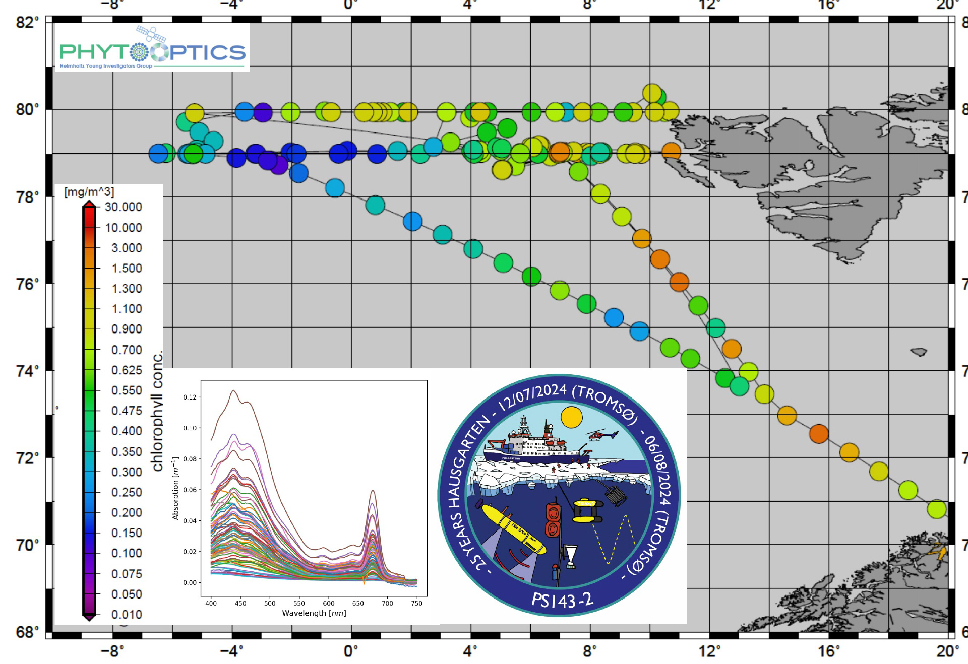
Die AWI-IUP Phytooptics-Gruppe nahm vom 12. Juli bis 5. August 2024 an der RV Polarstern-Expedition PS143-2 in der Framstraße (Ostgrönlandsee) teil, wo die Biodiversität und Biogeochemie des Oberflächenwassers im Vergleich zu den physikalischen Eigenschaften des Ozeans untersucht wurde.
Anhand optischer Messungen ermittelte die Phytooptics-Gruppe die spektrale Absorption von Unterwasserlicht durch Partikel im Allgemeinen und Phytoplankton im Besonderen. Erste Ergebnisse zeigen Messungen an Wasserproben, die mit der quantitativen Filtrationstechnik unter Verwendung eines integrativen Hohlraumabsorptionsmesssystems gemessen wurden (Details in Liu et al. 2018: https://doi.org/10.1364/OE.26.00A678)
Die Absorptionseigenschaften werden genutzt, um aus der spektralen Form und Stärke der Absorption die Zusammensetzung des Phytoplanktons zu bestimmen, hier wird aber auch die Gesamtbiomasse (Chlorophyllkonzentration) aus der Peakhöhe um 667 nm dargestellt. Während der östliche Teil höhere Konzentrationen aufweist, was mit dem Atlantikwasser in Verbindung gebracht wird, zeigt der westliche Teil eine sehr niedrige Chlorophyllkonzentration. Insgesamt ist die Biomasse nicht sehr hoch, was eher auf Bedingungen nach einer Algenblüte hindeutet.
Abbildung von Astrid Bracher (bracher@uni-bremen.de).
Juli 2024:
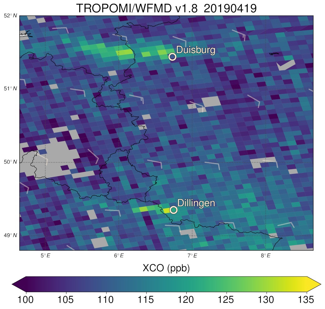
Die herkömmliche Stahlproduktion trägt aufgrund ihrer Abhängigkeit von kohlenstoffreichen Materialien wesentlich zu den weltweiten industriellen CO2-Emissionen bei. Um die Klimaziele zu erreichen, ist die systematische Dekarbonisierung der Stahlindustrie unerlässlich. Ein wichtiger Ansatz ist der Übergang zur wasserstoffbasierten Produktion, bei der Wasserdampf statt CO2 entsteht. Ein weiteres Nebenprodukt der konventionellen Stahlerzeugung ist Kohlenmonoxid (CO), das sich mit Satellitensensoren aus dem Weltraum besser überwachen lässt als das Treibhausgas CO2 selbst. Folglich kann mit emittiertes CO als wertvoller Indikator für den Kohlenstoff-Fußabdruck von Stahlwerken dienen.
Die Abbildung zeigt ein Beispiel für CO-Fahnen aus den beiden produktivsten Stahlwerken in Deutschland, die durch einen einzigen Überflug des TROPOspheric Monitoring Instrument (TROPOMI) an Bord des Sentinel-5 Precursor-Satelliten erfasst wurden. Durch eine systematische Langzeitauswertung der Satellitendaten lassen sich die CO-Emissionen aller deutschen integrierten Stahlwerke ermitteln (Schneising et al., 2024). Setzt man die geschätzten CO-Emissionen dieser Stahlproduktionsstandorte in Beziehung zu den von den Stahlherstellern für den gleichen Zeitraum gemeldeten zugehörigen CO2-Emissionen, so ergibt sich über alle analysierten Standorte hinweg eine sehr hohe Korrelation zwischen CO- und CO2-Emissionen. Diese lineare Beziehung rechtfertigt die Verwendung von CO als Proxy für die CO2-Emissionen vergleichbarer Stahlproduktionsstandorte, d. h. die Treibhausgasemissionen moderner konventioneller Stahlwerke können anhand der entsprechenden geschätzten CO-Emissionen und des auf deutsche Stahlwerke geeichten CO/CO2-Emissionsverhältnisses spezifisch aus dem Raum abgeleitet werden.
Referenz:
Schneising, O., Buchwitz, M., Reuter, M., Weimer, M., Bovensmann, H., Burrows, J. P., and Bösch, H.: Towards a sector-specific CO∕CO2 emission ratio: satellite-based observations of CO release from steel production in Germany, Atmos. Chem. Phys., 24, 7609–7621, https://doi.org/10.5194/acp-24-7609-2024, 2024.
Juni 2024:
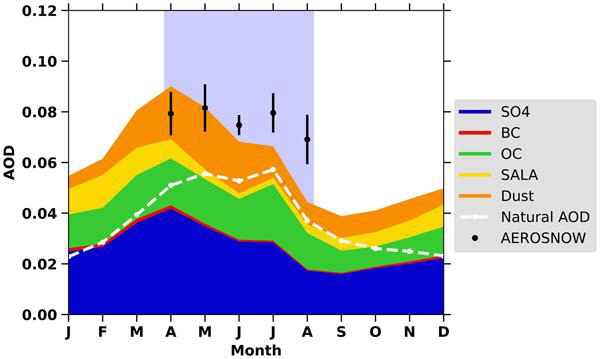
Aerosole sind kleine flüssige oder feste Schwebeteilchen in der Erdatmosphäre. Eine kürzlich von der IUP-Gruppe „Cloud Aerosol Surface PArameter Retrieval“ im Rahmen des transregionalen Projekts (AC)⊃3; durchgeführte Studie untersuchte die räumliche und zeitliche Verteilung von Aerosolen in der Arktis.
Arktische Aerosole sind wichtige Einflussfaktoren für das arktische Klima, da sie als Wolkenkondensationskerne oder eisbildende Partikel wirken können. Infolge ihrer unzureichend bekannten Verteilung und physikalisch-chemischen Charakterisierung sind auch die arktischen Wolken, die ihrerseits das arktische Klima stark beeinflussen, nur unzureichend bekannt.
Das Bild zeigt die Aerosol Optical Depth (AOD), ein Parameter, der die gesamte atmosphärische Aerosolbelastung beschreibt. Die AOD wird von Satellitenbeobachtungen abgeleitet und von GEOS-Chem, einem chemischen Transportmodell, modelliert. Die Satellitenbeobachtungen beruhen auf einem neuartigen Algorithmus, der von der Gruppe entwickelt und auf seine Qualität hin überprüft wurde. Andererseits spiegeln die Modellergebnisse den neuesten Stand des Verständnisses von Aerosolprozessen in der Arktis wider. Die Gegenüberstellung von satellitengestützten Beobachtungen und Modell wird uns daher zeigen, inwieweit unser (Modell-)Verständnis durch die Beobachtungen bestätigt wird oder nicht.
Die saisonale AOD über der zentralen arktischen Kryosphäre ist über den Zeitraum 2003-2011 gemittelt. Die gestapelte Darstellung zeigt das GEOS-Chem-Modell und die schwarzen Punkte die aus Satellitendaten abgeleitete mittlere AOD. Offensichtlich weichen die Modellergebnisse im Sommer von den Satellitendaten ab. Dies weist auf Schwächen des Modells in Bezug auf die Verteilung und Charakterisierung von Aerosolen im arktischen Sommer hin. Dies wiederum kann zu erheblichen Problemen bei der Charakterisierung der arktischen Wolken führen. Weitere Untersuchungen sind im Gange.
Referenz: Swain, B., Vountas, M., Singh, A., Anchan, N. L., Deroubaix, A., Lelli, L., Ziegler, Y., Gunthe, S. S., Bösch, H., and Burrows, J. P.: Aerosols in the central Arctic cryosphere: satellite and model integrated insights during Arctic spring and summer, Atmos. Chem. Phys., 24, 5671–5693, https://doi.org/10.5194/acp-24-5671-2024, 2024.
Kontakt/contact: Marco Vountas: vountas@iup.physik.uni-bremen.de
https://www.iup.uni-bremen.de/aerosol
Mai 2024:
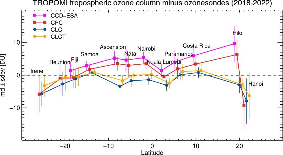
Die Breitenvariation der mittleren Differenz (md) und der Standardabweichung (sdev) zwischen der TROPOMI-Ozonsäule in der Troposphäre, die mit den vier Algorithmen, den ESA- (Europäische Weltraumorganisation, magenta) und unseren CPC- (rot), CLC- (blau) und CLCT- (gelb) Abfragen und den kollokierten Ozonsondensäulen im Zeitraum von 2018 bis 2022 abgerufen wurde.
Alle TROPOMI-Algorithmen verwenden die Convective-Cloud-Differential (CCD)-Methode, bei der von der Gesamtozonsäule am klaren Himmel die Säulenmenge über hohen konvektiven Wolken (Above-Cloud-Column-Ozon, ACCO) abgezogen wird, um die Ozonsäulenmengen in der Troposphäre (TrOC) zu erhalten. ESA und CPC verwenden ACCO nur aus der pazifischen Region, um TrOC über der gesamten tropischen Region zu erhalten, während die fortgeschrittenen Algorithmen CLC und CLCT ACCO aus nahe gelegenen Wolken verwenden (lokaler Wolkenalgorithmus). Die beiden letztgenannten Algorithmen führen zu einer besseren Übereinstimmung des troposphärischen Ozons von TROPOMI mit kollokierten Ozonsonden und machen diesen Algorithmus auch für die Anwendung in den Subtropen und Extratropen (z. B. in den mittleren Breiten) geeigneter. Troposphärisches Ozon ist ein starkes Treibhausgas und ein Schadstoff, der für unser Ökosystem schädlich ist. Globale Messungen des troposphärischen Ozons sind nur von Satelliteninstrumenten wie TROPOMI verfügbar.
Referenz: Maratt Satheesan, S., Eichmann, K.-U., Burrows, J. P., Weber, M., Stauffer, R., Thompson, A. M., and Kollonige, D.: Improved CCD tropospheric ozone from S5P TROPOMI satellite data using local cloud fields, EGUsphere [preprint], https://doi.org/10.5194/egusphere-2023-2825, 2024.
April 2024:
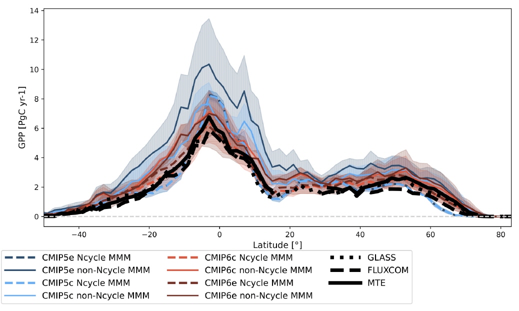
Unsere Abbildung des Monats zeigt die Bruttoprimärproduktion (GPP) aus Coupled Model Intercomparison Project Phase 6 (CMIP6; rot; Eyring et al, 2016) und CMIP5 (blau) Modellen mit (gestrichelt) und ohne (durchgezogen) interaktiven Stickstoffkreislauf (N-Kreislauf) im Vergleich zu Referenzdatensätzen, die auf Messungen des FLUXNET Eddy-Kovarianz-Turm-Netzwerks basieren: ein mit dem Model Tree Ensembles (MTE)-Ansatz hochskalierter Datensatz und FLUXCOM-Daten, die zusätzlich Moderate Resolution Imaging Spectroradiometer (MODIS) sowie meteorologische Daten unter Verwendung verschiedener maschineller Lernmethoden einbeziehen. Außerdem werden sowohl Simulationen mit vorgegebenen CO2-Emissionen (e, dunklere Farben) als auch mit vorgegebenen Konzentrationen (c, hellere Farben) verwendet. Die GPP stellt die CO2-Aufnahme an Land durch Photosynthese dar. Dies war eine der größten Schwächen des CMIP5-Ensembles, da die meisten Modelle die Photosynthese überschätzten. In der Abbildung ist dies an der starken Überschätzung des nicht-zyklischen CMIP5 im Vergleich zu den Referenzdatensätzen zu erkennen. Die CMIP6-MMMs ohne N-Zyklus zeigen eine viel bessere Annäherung in allen Breitengraden, mit einer leichten Verringerung der Verzerrung in den nördlichen Breiten, aber einer deutlichen Überschätzung in den Tropen. Die CMIP6-Ncycle-Modelle zeigen eine sehr gute Übereinstimmung mit den Referenzdaten in allen Breitengraden, jetzt mit leichten Unterschätzungen in hohen Breiten.
Diese Abbildung ist Teil von Gier et al. (2024), die Variablen des Kohlenstoffkreislaufs in CMIP6- und CMIP5-Simulationen untersucht und derzeit für Biogeosciences diskutiert wird. Gier et al. (2024) kommt zu dem Schluss, dass die Simulation der Photosynthese in Modellen mit Stickstoffkreislauf deutlich besser ist und dass es nur geringe Unterschiede zwischen emissions- und konzentrationsbasierten Simulationen gibt. Daher empfiehlt er, emissionsbasierte Simulationen in den kommenden CMIP7-Simulationen als Standardeinstellung zu verwenden und den Stickstoffkreislauf als notwendigen Bestandteil aller künftigen Kohlenstoffkreislaufmodelle zu betrachten.
Die Studie wurde vom Projekt Climate-Carbon Interactions in the Current Century (4C) unterstützt, das von der EU im Rahmen des Programms Horizon 2020 finanziert wird. Die Abbildung wurde mit dem Earth System Model Evaluation Tool v2 (ESMValTool; Eyring et al., 2020) erstellt. ESMValTool enthält viele Diagnosen zur Verwendung mit CMIP-Modellen und Beobachtungen sowie allgemeine Präprozessorfunktionen wie die Berechnung von Mittelwerten mehrerer Modelle, Gebietsmittelwerten und die Ableitung von benutzerdefinierten Variablen, die für diese Arbeit verwendet wurden.
Zugehörige Projekte:
Climate-Carbon Interactions in the Current Century (4C)
Coupled Model Intercomparison Project (CMIP)
REFERENZEN
Eyring, V., Bony, S., Meehl, G. A., Senior, C. A., Stevens, B., Stouffer, R. J., and Taylor, K. E.: Overview of the Coupled Model Intercomparison Project Phase 6 (CMIP6) experimental design and organization, Geosci Model Dev, 9, 1937-1958, 10.5194/gmd-9-1937-2016, 2016.
Eyring, V., Bock, L., Lauer, A., Righi, M., Schlund, M., Andela, B., Arnone, E., Bellprat, O., Brötz, B., Caron, L. P., Carvalhais, N., Cionni, I., Cortesi, N., Crezee, B., Davin, E. L., Davini, P., Debeire, K., de Mora, L., Deser, C., Docquier, D., Earnshaw, P., Ehbrecht, C., Gier, B. K., Gonzalez-Reviriego, N., Goodman, P., Hagemann, S., Hardiman, S., Hassler, B., Hunter, A., Kadow, C., Kindermann, S., Koirala, S., Koldunov, N., Lejeune, Q., Lembo, V., Lovato, T., Lucarini, V., Massonnet, F., Müller, B., Pandde, A., Pérez-Zanón, N., Phillips, A., Predoi, V., Russell, J., Sellar, A., Serva, F., Stacke, T., Swaminathan, R., Torralba, V., Vegas-Regidor, J., von Hardenberg, J., Weigel, K., and Zimmermann, K.: Earth System Model Evaluation Tool (ESMValTool) v2.0 – an extended set of large-scale diagnostics for quasi-operational and comprehensive evaluation of Earth system models in CMIP, Geosci. Model Dev., 13, 3383-3438, 10.5194/gmd-13-3383-2020, 2020.
Gier, B. K., Schlund, M., Friedlingstein, P., Jones, C. D., Jones, C., Zaehle, S., and Eyring, V.: Representation of the Terrestrial Carbon Cycle in CMIP6, EGUsphere [preprint], https://doi.org/10.5194/egusphere-2024-277, 2024.
März 2024:
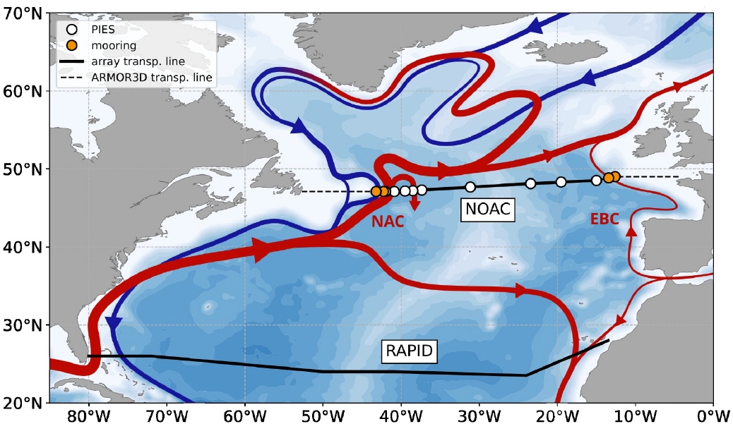
Da Klimamodellstudien für das 21. Jahrhundert einen Rückgang der atlantischen meridionalen Umwälzzirkulation (AMOC) voraussagen, ist die Überwachung der AMOC-Veränderungen nach wie vor unerlässlich. Es wird erwartet, dass die AMOC-Variabilität über Breitengrade hinweg auf längeren als dekadischen Zeitskalen kohärent ist, während die Konnektivität auf zwischenjährlichen und saisonalen Zeitskalen weniger eindeutig ist. Modellstudien und Beobachtungsschätzungen stimmen nicht über die Regionen und Zeitskalen der meridionalen Konnektivität überein, und AMOC-Beobachtungen in mehreren Breitengraden sind erforderlich, um die Konnektivität zu untersuchen. Wir berechnen den beckenweiten AMOC-Volumentransport (1993-2018) anhand von Messungen des Arrays North Atlantic Changes (NOAC) auf 47°N und kombinieren Daten von verankerten Instrumenten mit Hydrographie und Satellitenaltimetrie. Die mittlere NOAC AMOC beträgt 17,2\,Sv und zeigt keinen langfristigen Trend. Sowohl die ungefilterte als auch die tiefpassgefilterte NOAC-AMOC zeigen eine signifikante Korrelation mit der RAPID-MOCHA-WBTS-AMOC auf 26°N, wobei die NOAC-AMOC um etwa ein Jahr voraus ist.
Mehr Information:
Wett, S., M. Rhein, D. Kieke, C. Mertens, und M. Moritz (2023), Meridional connectivity of a 25-year observational AMOC record at 47°N. Geophysical Research Letters, 50, e2023GL103284, doi:10.1029/2023GL103284.
Februar 2024:
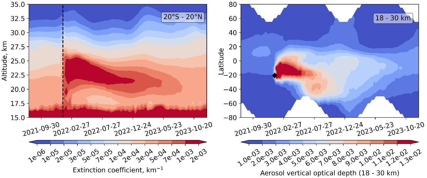
Vertikale Verteilungen des stratosphärischen Aerosol-Extinktionskoeffizienten wurden an der Universität Bremen aus Messungen des gestreuten Sonnenlichts in der Limb-Viewing-Geometrie mit dem OMPS-LP-Instrument der NASA/NOAA gewonnen. Die gewonnenen Daten ermöglichen es uns, die Entwicklung der Aerosolfahne nach dem Ausbruch des Hunga Tonga-Hunga Haʻapai Vulkans im Januar 2022 zu untersuchen.
Das linke Feld zeigt die zonale Verteilung des mittleren Aerosolextinktionskoeffizienten in den Tropen. Das Maximum der Abgasfahne erreichte eine Höhe von etwa 26 km und blieb bis Mitte Mai 2022 in dieser Höhe. Danach ist ein schnelles Absinken des Fahnenmaximums zu beobachten. Das rechte Feld zeigt die vertikale optische Tiefe des stratosphärischen Aerosols (18 - 30 km). Die Abgasfahne breitete sich hauptsächlich auf der südlichen Hemisphäre aus. Einige Transportvorgänge in die nördliche Hemisphäre sind ebenfalls zu beobachten, z. B. Ende 2022. Am Ende des analysierten Datensatzes (Dezember 2023) werden in den Tropen und den südlichen mittleren Breiten immer noch erhöhte Werte für die optische Tiefe des stratosphärischen Aerosols beobachtet.