

Bild des Monats 2020 - 2021
Dezember 2021:
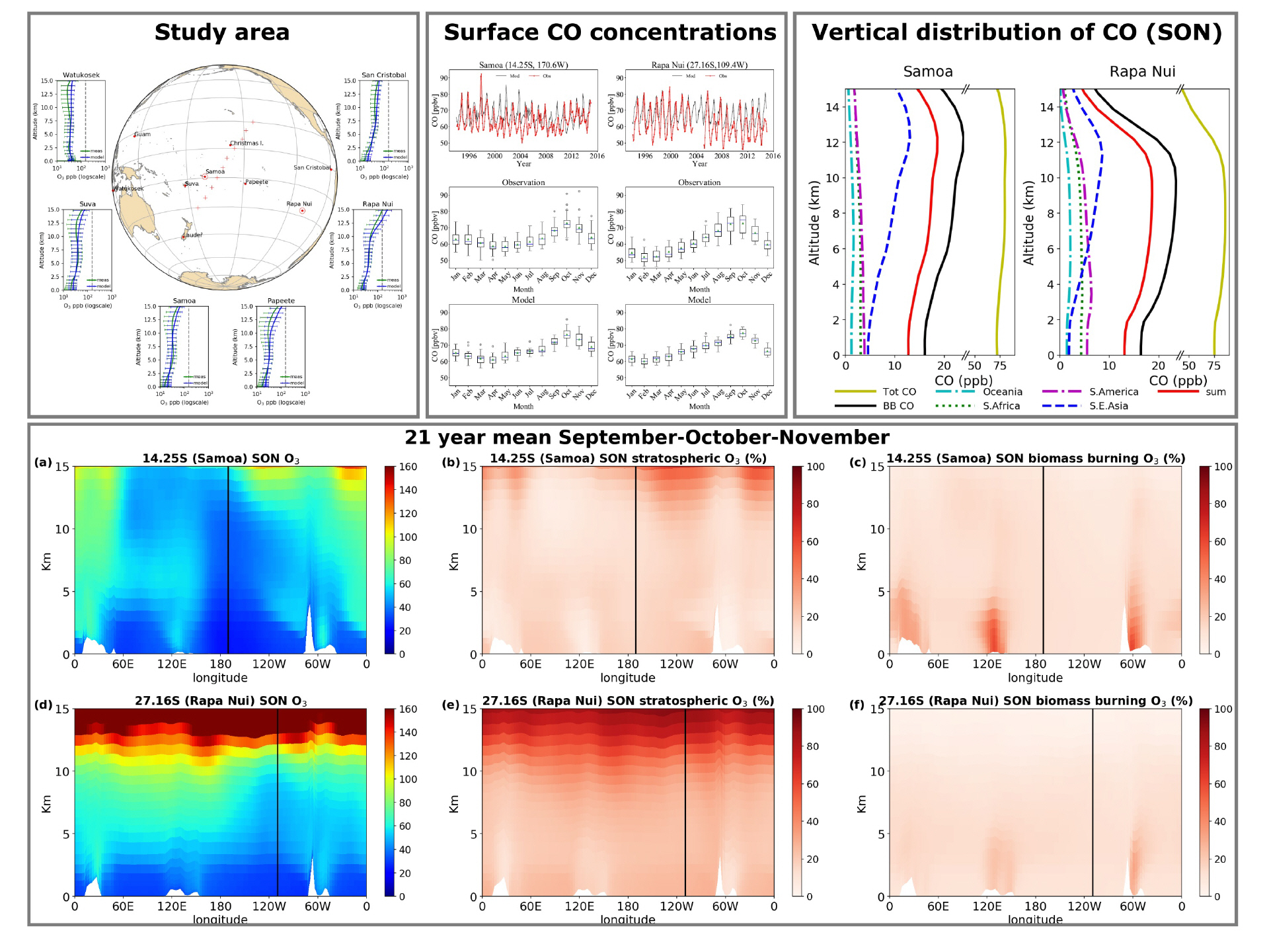
The importance of Biomass Burning carbon monoxide on the O3 concentrations in the remote southern Pacific Ocean. (Based on: Impact of biomass burning and stratospheric intrusions in the remote South Pacific Ocean troposphere, Nikos Daskalakis et al., ACP, 2021)
Top left: Area of study, with locations of CO (crosses) and O3 (dots) measurements, with average O3 concentrations from ozonesondes (green lines) and from the TM4-ECPL model (blue lines) for the years 1994-2014.
Top center: Time series and box and whisker plots of surface CO concentrations from measurements and model at Samoa and Rapa Nui.
Top right: Vertical distribution of CO originating from biomass burning from different regions, as simulated over Samoa and Rapa Nui.
Bottom: O3 concentrations at the cross section at the latitude of Samoa (a) and Rapa Nui (d), percentage contribution of stratospheric tropospheric exchange on O3 at the latitude of Samoa (b) and Rapa Nui (e) and percentage contribution of biomass burning on O3concentrations at the latitude of Samoa (c) and Rapa Nui (f).
Ozone (O3) is a secondary pollutant in the global troposphere, produced through chemistry from its precursors. One of the main precursors of O3 is carbon monoxide (CO), that is mainly primarily emitted from incomplete burning. Wildfires biomass burning is a major CO emitter. Wildfires happen every year all around the globe, impacting, among others, the chemical composition of the local atmosphere (where the fire happens), but also the global atmosphere, through transport of pollution.
In this work we study the impact of biomass burning originating from different regions of the world (namely the source regions as defined by the HTAP, Galmarini et al, 2017, HTAP, 2010), on the remote southern Pacific Ocean O3 concentrations, represented by two locations, one in the west (Samoa) and one in the East (Rapa Nui) (top left figure). In this study we used i) TM4-ECPL simulations run for the period 1994-2014, to capture the long term tendencies of transport and concentrations, as well as ii) in-situ observations at the aforementioned locations (top center and top right figures).
We found that even the most remote region of the world can be impacted by the pollution emitted from wildfires, producing O3. The impact, during the southern hemispheric burning season (September-October-November) is bigger closer to the equator, and closer to the surface, as shown in the bottom figure. As we move to the south, the impact of wildfires O3 is masked by the increased tropospheric-stratospheric exchange of O3.
References
Daskalakis, N., Gallardo, L., Kanakidou, M., Nüß, R., Menares, C., Rondanelli, R., Thompson, A. M., and Vrekoussis, M.: Impact of biomass burning and stratospheric intrusions in the remote South Pacific Ocean troposphere, Atmos. Chem. Phys. Discuss. [preprint], https://doi.org/10.5194/acp-2021-640, in review, 2021.
Galmarini, S., Koffi, B., Solazzo, E., Keating, T., Hogrefe, C., Schulz, M., Benedictow, A., Jurgen Griesfeller, J., Janssens-Maenhout, G., Carmichael, G., Fu, J. and Dentener, F.: Technical note: Coordination and harmonization of the multi-scale, multi-model activities HTAP2, AQMEII3, and MICS-Asia3: Simulations, emission inventories, boundary conditions, and model output formats, Atmos. Chem. Phys., 17(2), 1543–1555, doi:10.5194/acp-17-1543-2017, 2017.
HTAP: Hemispheric Transport of Air Pollution 2010, PART A: OZONE AND PARTICULATE MATTER, ECONOMIC C., edited by H. Dentener, F., Keating, T., and Akimoto, UNITED NATIONS PUBLICATION, Geneva, Switzerland. [online] Available from: http://www.htap.org/publications/2010_report/2010_Final_Report/HTAP 2010 Part A 110407.pdf, 2010.
November 2021:
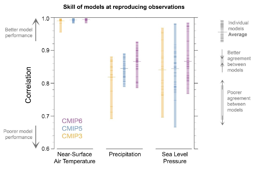
Our picture of the month shows one of our several contributions to the IPCC Sixth Assessment Report (AR6) based on work done by the IUP Climate Modelling department in collaboration with the department of “Earth System Model Evaluation and Analysis” at the DLR Institute of Atmospheric Physics in Oberpfaffenhofen. Here, three generations of CMIP (Coupled Model Intercomparison Project) models are compared to observations using pattern correlations for annual mean climatology, calculated for the period 1980 to 1999, of surface air temperature, precipitation, and sea level pressure. The short horizontal lines show the results for individual models from CMIP3 (orange), CMIP5 (blue), and CMIP6 (purple), the longer horizontal lines show the multi-model average of all models of the same generation. The multi-model average indicates an increasing correlation from CMIP3 to CMIP6, which points towards an improved performance of the later model generations. The shown plot is included in the frequently asked questions (FAQ) section of Chapter 3 “Human Influence on the Climate System” of the IPCC AR6 Working Group I report (Eyring et al. 2021) and is based on Bock et al. (2020).
The Working Group I contribution to AR6, “The Physical Science Basis” (IPCC 2021) was published on 9 August 2021 of which Prof. Veronika Eyring is one of Chapter 3’s coordinating lead authors. The report concludes that it is unequivocal that human influence has warmed the atmosphere, ocean and land. Widespread and rapid changes in the Earth system have occurred and are unprecedented over thousands of years. It also shows that unless there are immediate, rapid, and large-scale reductions in greenhouse gas emissions, limiting warming to 1.5°C will be beyond reach (IPCC, 2021). The analysis of climate model simulations in several chapters of the report was facilitated by the ESMValTool (Earth System Model Evaluation Tool, Eyring et al. 2020; Lauer et al. 2020; Righi et al. 2020; Weigel et al. 2021). The ESMValTool is developed in a collaboration with 70 international research institutions including the Climate Modelling department at IUP.
Prof. Veronika Eyring was awarded the Gottfried Wilhelm Leibniz Prize 2021 earlier this year for her significant contribution to improve the understanding and accuracy of climate predictions through process-oriented modeling and model evaluation. Her research focuses on Earth system modeling and process-oriented model evaluation and analysis, including artificial intelligence (AI) techniques, to improve climate projections and technology assessments.
Related projects:
Advanced Earth System Model Evaluation for CMIP (Eval4CMIP)
Climate-Carbon Interactions in the Current Century (4C)
Coupled Model Intercomparison Project (CMIP)
Further reading:
Bock, L., Lauer, A., Schlund, M., Barreiro, M., Bellouin, N., Jones, C., Meehl, G.A., Predoi, V., Roberts, M.J., & Eyring, V. (2020). Quantifying Progress Across Different CMIP Phases With the ESMValTool. Journal of Geophysical Research-Atmospheres, 125
Eyring, V., Bock, L., Lauer, A., Righi, M., Schlund, M., Andela, B., Arnone, E., Bellprat, O., Brötz, B., Caron, L.P., Carvalhais, N., Cionni, I., Cortesi, N., Crezee, B., Davin, E.L., Davini, P., Debeire, K., de Mora, L., Deser, C., Docquier, D., Earnshaw, P., Ehbrecht, C., Gier, B.K., Gonzalez-Reviriego, N., Goodman, P., Hagemann, S., Hardiman, S., Hassler, B., Hunter, A., Kadow, C., Kindermann, S., Koirala, S., Koldunov, N., Lejeune, Q., Lembo, V., Lovato, T., Lucarini, V., Massonnet, F., Müller, B., Pandde, A., Pérez-Zanón, N., Phillips, A., Predoi, V., Russell, J., Sellar, A., Serva, F., Stacke, T., Swaminathan, R., Torralba, V., Vegas-Regidor, J., von Hardenberg, J., Weigel, K., & Zimmermann, K. (2020). Earth System Model Evaluation Tool (ESMValTool) v2.0 – an extended set of large-scale diagnostics for quasi-operational and comprehensive evaluation of Earth system models in CMIP. Geosci. Model Dev., 13, 3383-3438
Eyring, V., Gillett, N.P., Achuta Rao, K.M., Barimalala, R., Barreiro Parrillo, M., Bellouin, N., Cassou, C., Durack, P.J., Kosaka, Y., McGregor, S., Min, S., Morgenstern, O., & Sun, Y. (2021). Human Influence on the Climate System. In Climate Change 2021: The Physical Science Basis. . In V. Masson-Delmotte, P. Zhai, A. Pirani, S.L. Connors, C. Péan, S. Berger, N. Caud, Y. Chen, L. Goldfarb, M.I. Gomis, M. Huang, K. Leitzell, E. Lonnoy, J.B.R. Matthews, T.K. Maycock, T. Waterfield, O. Yelekçi, R. Yu, & B. Zhou (Eds.), Contribution of Working Group I to the Sixth Assessment Report of the Intergovernmental Panel on Climate Change. Cambridge University Press. In Press.
IPCC (2021). Climate Change 2021: The Physical Science Basis. https://www.ipcc.ch/report/ar6/wg1/. In V. Masson-Delmotte, P. Zhai, A. Pirani, S.L. Connors, C. Péan, S. Berger, N. Caud, Y. Chen, L. Goldfarb, M.I. Gomis, M. Huang, K. Leitzell, E. Lonnoy, J.B.R. Matthews, T.K. Maycock, T. Waterfield, O. Yelekçi, R. Yu, & B. Zhou (Eds.), Contribution of Working Group I to the Sixth Assessment Report of the Intergovernmental Panel on Climate Change. Cambridge University Press. In Press.
Lauer, A., Eyring, V., Bellprat, O., Bock, L., Gier, B.K., Hunter, A., Lorenz, R., Perez-Zanon, N., Righi, M., Schlund, M., Senftleben, D., Weigel, K., & Zechlau, S. (2020). Earth System Model Evaluation Tool (ESMValTool) v2.0-diagnostics for emergent constraints and future projections from Earth system models in CMIP. Geoscientific Model Development, 13, 4205-4228
Righi, M., Andela, B., Eyring, V., Lauer, A., Predoi, V., Schlund, M., Vegas-Regidor, J., Bock, L., Brötz, B., de Mora, L., Diblen, F., Dreyer, L., Drost, N., Earnshaw, P., Hassler, B., Koldunov, N., Little, B., Loosveldt Tomas, S., & Zimmermann, K. (2020). Earth System Model Evaluation Tool (ESMValTool) v2.0 – technical overview. Geosci. Model Dev., 13, 1179-1199
Weigel, K., Bock, L., Gier, B.K., Lauer, A., Righi, M., Schlund, M., Adeniyi, K., Andela, B., Arnone, E., Berg, P., Caron, L.P., Cionni, I., Corti, S., Drost, N., Hunter, A., Lledo, L., Mohr, C.W., Pacal, A., Perez-Zanon, N., Predoi, V., Sandstad, M., Sillmann, J., Sterl, A., Vegas-Regidor, J., von Hardenberg, J., & Eyring, V. (2021). Earth System Model Evaluation Tool (ESMValTool) v2.0-diagnostics for extreme events, regional and impact evaluation, and analysis of Earth system models in CMIP. Geoscientific Model Development, 14, 3159-3184
Oktober 2021:
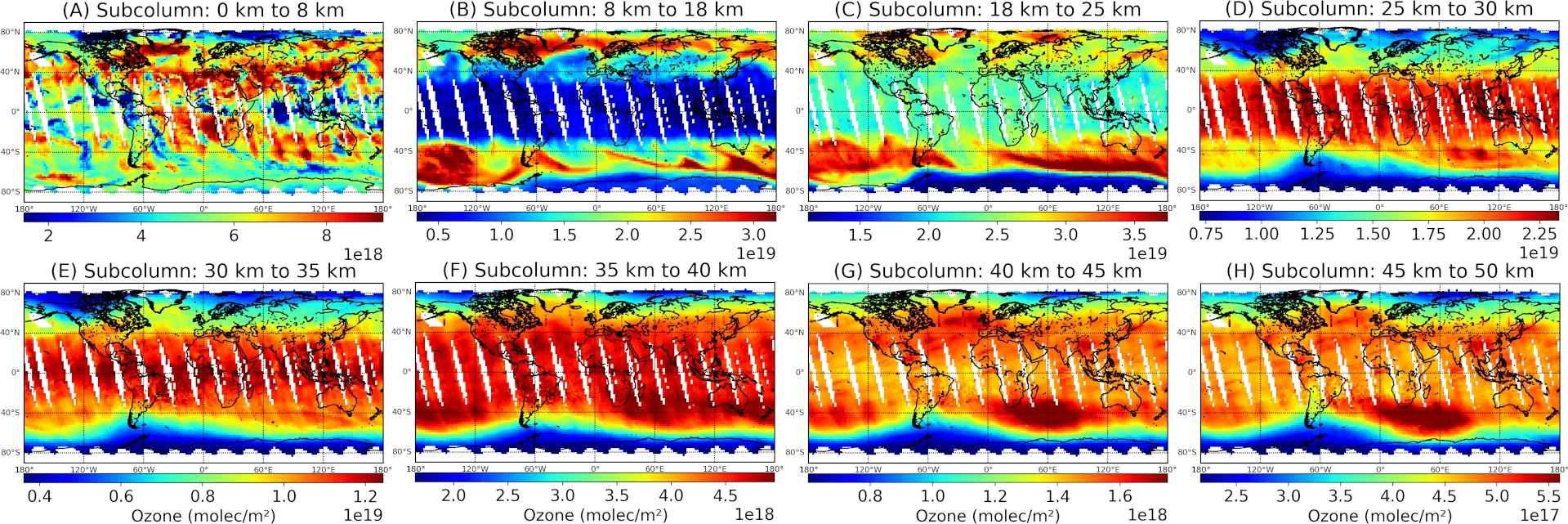
Observing ozone is a key point for studying the chemistry and dynamics of the atmosphere, as well as for monitoring greenhouse gases and climate change. Since ozone is not homogeneously distributed in the atmosphere and has different roles in different atmospheric layers, it is also important to have profile information. In this study we retrieved ozone profiles from radiation measurements in the ultraviolet spectral range (270 - 329 nm) of the TROPOMI nadir-viewing instrument aboard the Sentinel-5 Precursor (S5P) satellite.
S5P is the latest member of the European family of combined ozone and greenhouse gas monitoring satellites and was launched in 2017. It allows retrieving ozone profiles globally with high spatial resolution on a single day. This figure shows our TOPAS (Tikhonov regularized Ozone Profile retrievAl with SCIATRAN) ozone profiles from 1 October 2018. The vertical resolution is less than 9 km above 18 km but much lower below 18 km. The panels with the different subcolumns show the spatial and vertical ozone distribution. The ozone peak in the stratosphere (“the ozone layer”, panels C and D) and the Antarctic ozone hole can be seen. In the lower troposphere (panel A) the scattering is somewhat larger and clouds influence the results.
The typical tropospheric ozone maximum over the South Atlantic and South Africa is observed. We validated our results with ozonesondes and stratospheric lidars and found an accuracy of ±5% in the stratosphere (except at very high latitudes). The results also agree to within ±10 % in the troposphere, but the standard deviation is high. An excellent agreement was found when comparing with ozone profiles from other limb-viewing satellites (MLS and OMPS).
Further reading:
Mettig, N., Weber, M., Rozanov, A., Arosio, C., Burrows, J. P., Veefkind, P., Thompson, A. M., Querel, R., Leblanc, T., Godin-Beekmann, S., Kivi, R., and Tully, M. B.: Ozone profile retrieval from nadir TROPOMI measurements in the UV range, Atmos. Meas. Tech., 14, 6057–6082, https://doi.org/10.5194/amt-14-6057-2021, 2021.
September 2021:
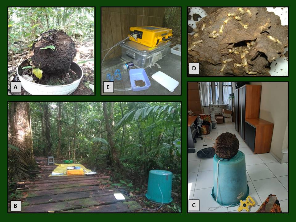
The measurement of termite CH4 emission in a tropical rainforest
Termites are insects that are highly abundant in tropical ecosystems. It is known that termites emit methane (CH4), an important greenhouse gas, but their absolute emission remains uncertain.
As part of the DFG project ‘Methane fluxes from seasonally flooded forests in the Amazon basin’, and in collaboration with the institute LBA-INPA (Manaus, Amazonas, Brazil), IUP Bremen initiated CH4 flux measurements in a pristine tropical rainforest, at a field site close to Manaus. As part of this project, the CH4 emission of termites and termite mounds (nests) of the species ‘Neocapritermes brasiliensis’ were studied.
The emission of termite mounds was measured by placing a large flux chamber (bucket) over the mound, and continuously measuring the CH4 concentrations in the flux chamber by use of a portable analyzer. By using data from local ecology and entomology studies, it could be estimated how much methane was emitted by termite mounds in this ecosystem.
In addition, we measured the emission of different nest pieces, and afterwards counted the individual termites. By use of this method, we could determine a termite emission factor (average CH4 emission per gram termite), which can be used to upscale termite emission to ecosystem or global scale.
In this ecosystem, we found that termites emit around ~1 nmol m−2 s−1, and thereby play a crucial role in the CH4 budget of this ecosystem.
Explanation of photos: A) Termite mound (nest) of the species N. brasiliensis, B) CH4 flux measurement of mound in field by use of a portable instrument (yellow suitcase) and flux chamber (large bucket), C) Sampling of complete termite nest for further study in the laboratory, D) Individual termites in nest piece, E) CH4 emission measurement of individual nest pieces.
Further reading:
van Asperen, H., Alves-Oliveira, J. R., Warneke, T., Forsberg, B., de Araújo, A. C., and Notholt, J.: The role of termite CH4 emissions on the ecosystem scale: a case study in the Amazon rainforest, Biogeosciences, 18, 2609–2625, https://doi.org/10.5194/bg-18-, 2021.
August 2021:
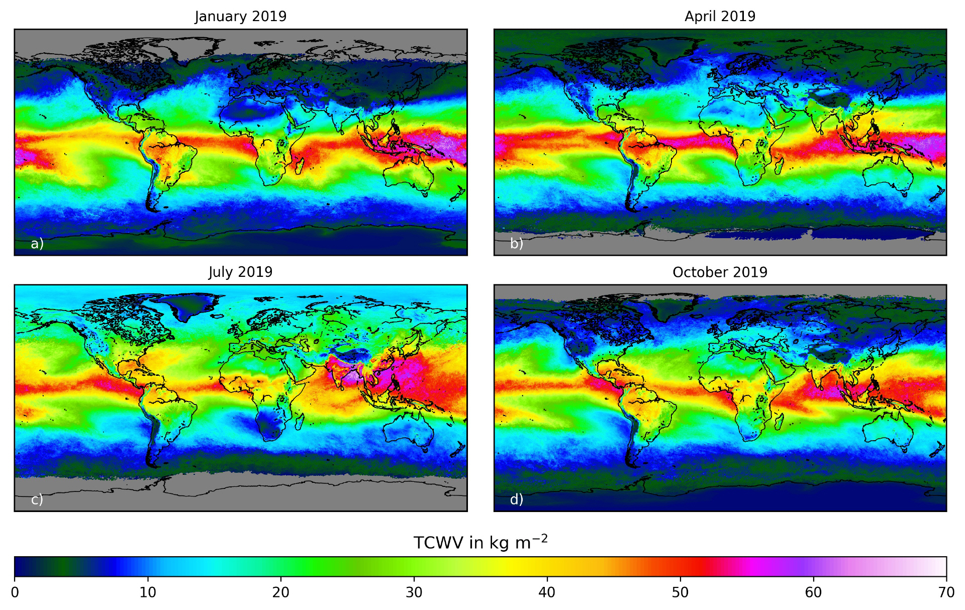
Globale Wasserdampfverteilungen aus Satellitendaten
Der Wasserdampf in der Atmosphäre spielt bei vielen Prozessen eine Schlüsselrolle. Wie Kohlendioxid und andere Treibhausgase ist er in der Lage, Wärmestrahlung an die Erdoberfläche zurück zu emittieren. Wenn Wasserdampf kondensiert, bilden sich Wolken, die ebenso den Strahlungshaushalt der Erde beeinflussen. Quellen des Wasserdampfes sind alle Wasseroberflächen sowie Vegetation und feuchter Boden auf dem Land. Einige der Wolken bringen Niederschläge mit sich, die teilweise von der Oberfläche abfließen und Flüsse bilden. Dieser Kreislauf von Verdunstung, Niederschlag und Abfluss bildet den sogenannten Wasserkreislauf.
Der Wasserdampf in der Atmosphäre kann durch Satellitenmessungen über den gesamten Globus beobachtet werden. Die Abbildung (veröffentlicht in Küchler et al., 2021) zeigt eine globale Karte des monatlich gemittelten Gesamtwasserdampfgehaltes der Atmosphäre, welcher am Institut für Umweltphysik aus Sentinel-5Precursor-Daten erstellt wurde.
Der höchste Wasserdampfgehalt ist über tropischen Regionen zu sehen. In Richtung der geografischen Pole nimmt die Wasserdampfmenge ab. Dies ist auf die niedrigere Temperatur zurückzuführen. Über den Polarregionen gibt es im Winter aufgrund des fehlenden Sonnenlichts keine Daten, die zur Ermittlung der Gesamtwasserdampfsäule benötigt werden.
Die jährliche Änderung der Wasserdampfsäule ist durch den Vergleich der Abbildungen a-d ersichtlich. Die meisten Merkmale folgen dem Sonnenstand, z.B. die Innertropische Konvergenzzone mit den höchsten Gesamtwasserdampfsäulen. Große Änderungen sind über den mittleren Breiten von Januar bis Juli aufgrund des Temperaturwechsels vom Winter zum Sommer zu sehen. Auch Indien zeigt große Veränderungen des Wasserdampfes aufgrund der Monsunzirkulation.
Normalerweise erhalten Wüsten wie die Sahara nur sehr wenig Niederschlag bis zu wenigen mm pro Jahr. Dennoch gibt es vor allem im Sommer und Herbst etwa 20 mm Gesamtwasserdampfsäule.
Referenz:
Küchler, T., Noël, S., Bovensmann, H., Burrows, J. P., Wagner, T., Borger, C., Borsdorff, T., and Schneider, A.: Total water vapour columns derived from Sentinel 5p using the AMC-DOAS method, Atmos. Meas. Tech. Discuss. [preprint], https://doi.org/10.5194/amt-2021-144, in review, 2021.
Contact:
Tobias Küchler (tobias.kuechler@iup.physik.uni-bremen.de)
Stefan Noël (stefan.noel@iup.physik.uni-bremen.de)
Juli 2021:
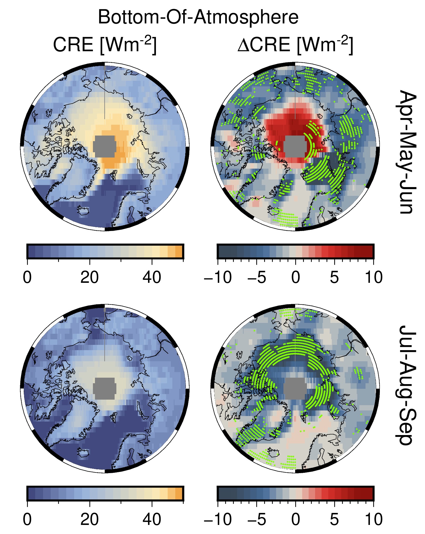
Arktische Wolken sind ein wichtiger Faktor in der Beeinflussung des arktischen Klimas. Sie wirken dabei sowohl erwärmend als auch abkühlend. Die Gründe wann sie erwärmend oder abkühlend wirken hängen von verschiedenen Bedingungen ab. Hierzu gehören die mikrophysikalischen Eigenschaften der Wolken, die Beleuchtung, die thermodynamische Phase der Wolken (also bis zu welchem Grad sie flüssig oder gefrorenes Wasser beinhalten) und die Reflektivität des Bodens.
Eine jüngst von der IUP Gruppe „Cloud Aerosol Surface Parameter Retrieval“ im Rahmen des Transregios (AC)⊃3; durchgeführte Studie untersucht die Wolken, ihre Eigenschaften und die Größe des Strahlungseffektes (Cloud Radiative Effect - CRE) von Wolken auf der Basis von 20 Jahren an Satellitendaten. Ist der CRE positiv, so wärmen die Wolken, ist er negativ wirken die Wolken kühlend. Auf dem Bild sieht man, dass die Wolken im Frühling wie auch im Sommer die Oberfläche immer wärmen. Allerdings sieht man auch, dass der Erwärmungseffekt im Frühling vor allem in Regionen wo die Eisbedeckung deutlich abnimmt sehr zunimmt (∆CRE > 0), ansonsten aber auch ein gegenläufiger Trend begonnen hat. Diesen gegenläufigen Trend beobachten wir auch im Sommer (blaue Regionen).
Reference:
The aerosol, cloud and surface property group "Pan-Arctic and regional trends of reflectance, clouds and fluxes: implications for Arctic Amplification" (2021)
Kontakt/contact: Marco Vountas
vountas@iup.physik.uni-bremen.de
https://www.iup.uni-bremen.de/aerosol
Juni 2021:
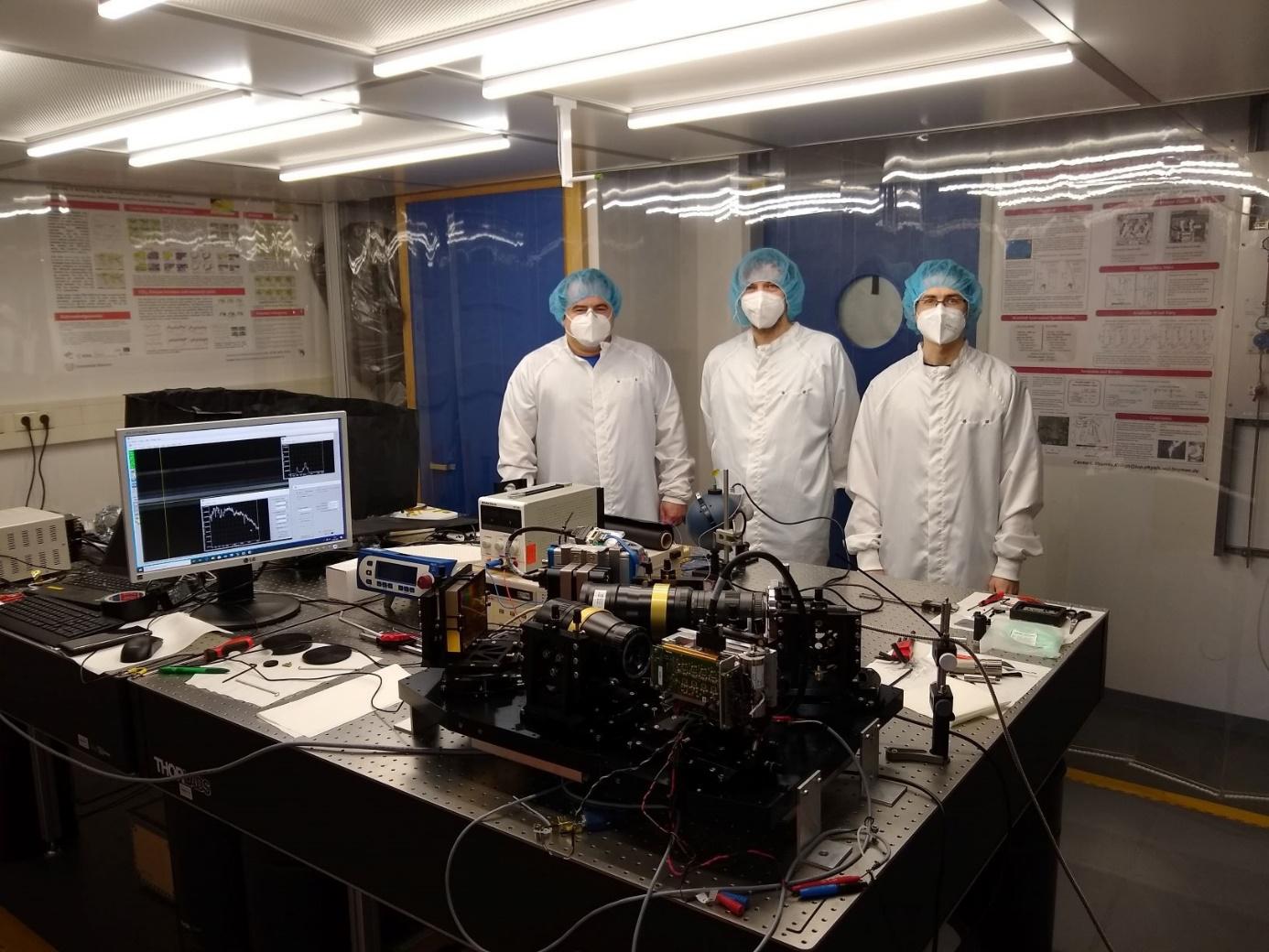
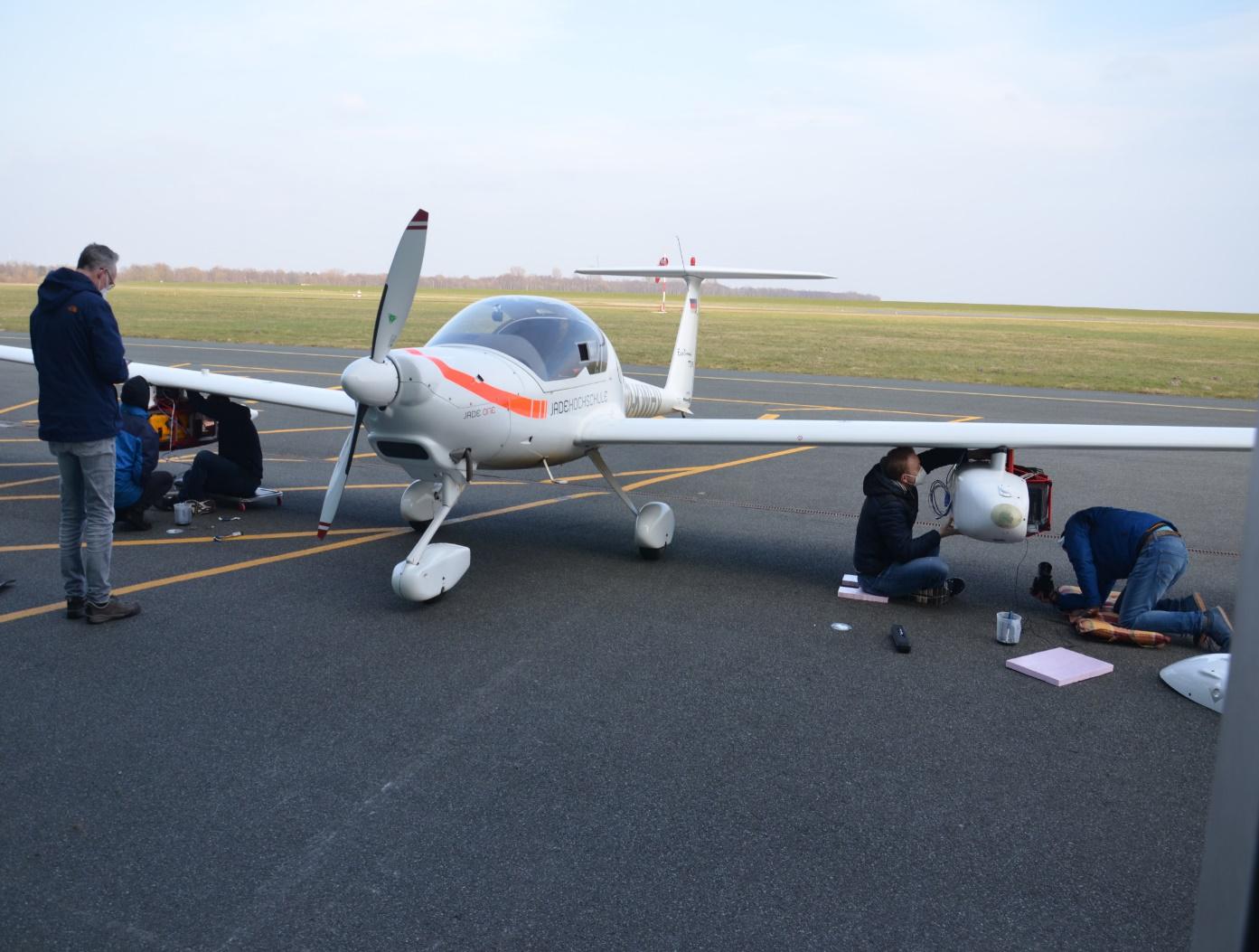
New sensor to image Methane from aircraft under development at IUP, University Bremen
Scientists of the Institute of Environmental Physics are developing a new optical sensor to image atmospheric Methane (CH4) and CO2 distributions from aircraft in a similar way as future satellites, but with higher sensitivity to point source emissions. The prototype (or “flying breadboard”) of the push broom imaging spectrometer – called MAMAP 2D Lite - is currently under test in the laboratory and from aircraft. The sensor was mounted in the wing pods of the motor glider of Jade Hochschule Wilhelmshaven and was deployed successfully for an initial functional test. Next step is the test of the system at different Methane and CO2 targets, to assess, optimise and document the sensor performance and data analysis methods.
After that, the full system - MAMAP2D - comprising two imaging spectrometer with high fidelity custom made cameras will be integrated and tested. The full system will be ready in summer 2022 for a measurement campaign in North America and Canada using the German high altitude research aircraft HALO, as part of an international measurement campaign to better understand northern wetland emissions as well as high latitude emissions from geological seeps and oil/gas production.
Contact: heinrich.bovensmann@uni-bremen.de
Mai 2021:
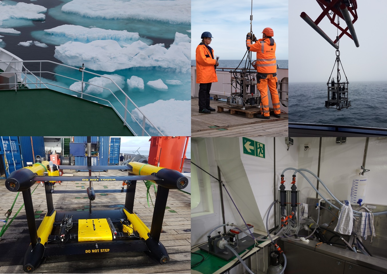
Image of May 2021: The AWI-IUP Phytooptics group’s research enables the continuous survey of the underwater light field, and of the particle and phytoplankton composition and distribution. The image shows the group’s measurements taken during expedition MSM93 onboard RV Maria S. Merian at the Arctic Ocean (Fram Strait) via operating hyperspectral active and passive bio-optical instruments (Photos: Julia Oelker (IUP & AWI), Tim Kalvelage):
To measure actively the absorption and attenuation of the water constituents in the upper ocean resolved for the different depth layers down to 100 -150 m two Wetlabs/Seabird instruments ACS are operated on a steel frame lowered by the ship’s winch at discrete stations (upper two right figures) and towed behind the ship on an undulating platform (lower left figure). To permanently measure during the entire expedition these properties also specifically for the particles, another ACS instrument is operated with surface water pumped via a flow-through setup in the ship’s laboratory (lower right figure). Via radiometers mounted (with the ACS) to the steel frame (upper right figures) and to the undulating platform (lower left figure), corrected for the incident sunlight measured by another radiometer (upper left figure), the underwater light profile spectrally is determined. Several algorithms have been developed and have been applied to obtain from these optical data the spectral characteristics of the underwater light field and the abundance and composition of its optical constituents (dissolved organic matter, phytoplankton and other particles). These data are further used to calculate primary production or pre-cursors of biogenic emissions. For more information, have a look at the group’s publications at https://www.awi.de/index.php?id=2556&L=1 .
April 2021:
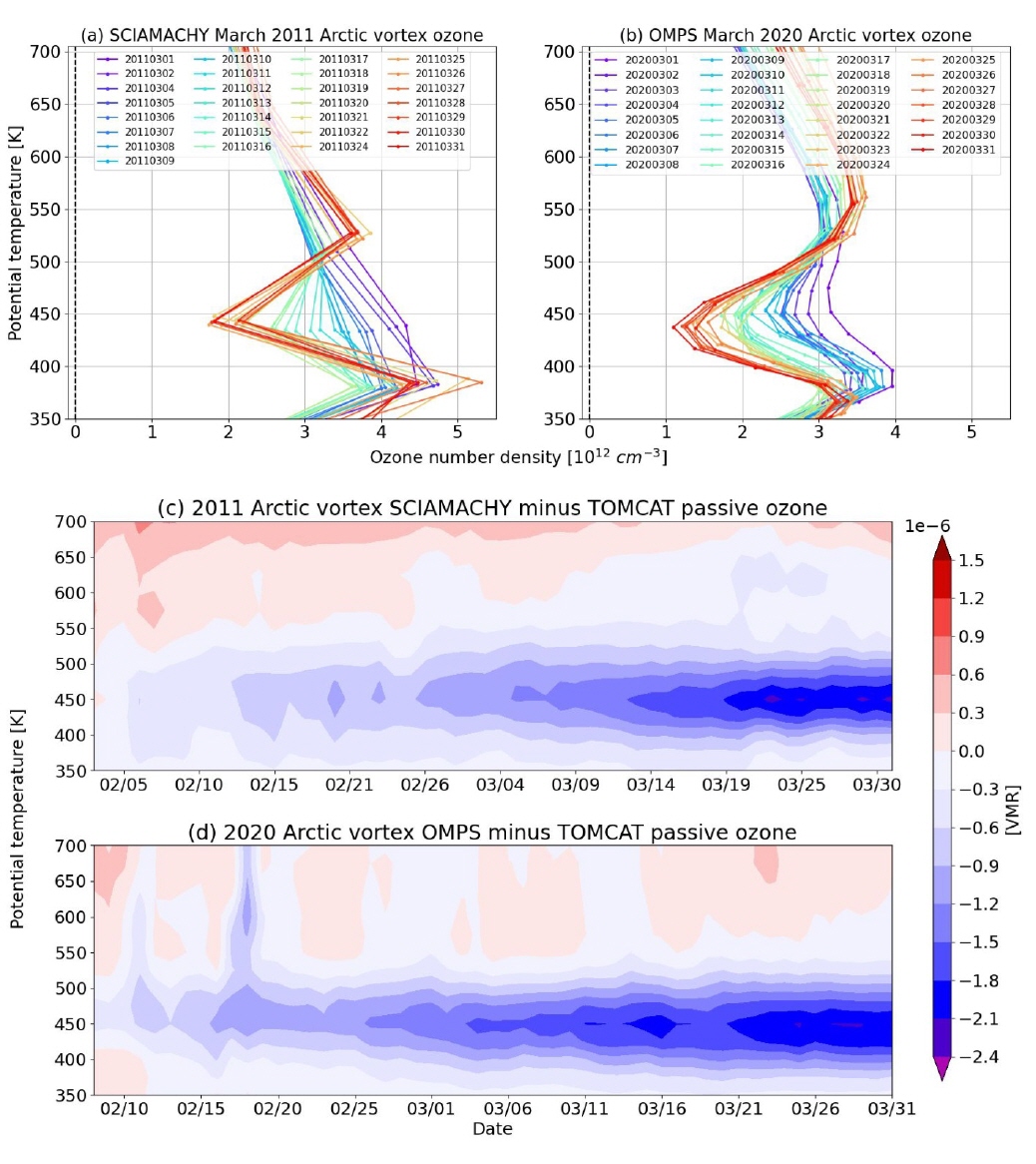
During winter/spring 2019/20 in the Arctic very low stratospheric temperatures were recorded, associated with an extensive formation of polar stratospheric clouds and a strong depletion of ozone, particularly during March. Total ozone was up to 200 DU lower than the year before, reaching values comparable with the ones in the Antarctic ozone hole. This event was similar to the low ozone recorded in 2010/11 (Manney et al., 2011). An investigation of this event in comparison with 2010/11 was performed using satellite limb observations from SCIAMACHY and OMPS-LP, together with simulations from the TOMCAT chemistry transport model (CTM).
The figure, in panel (a) and (b), shows the time series of March daily mean vortex-averaged ozone profiles from SCIAMACHY (2011) and OMPS-LP (2020) respectively. Ozone profiles with a potential vorticity (PV) value higher than 38 PVU (at 475 K) were averaged to obtain the daily profiles. In both cases we observe throughout March a rapid decline of ozone near 450 K potential temperature level, which corresponds to ~18 km altitude. The very stable polar vortex and the extensive formation of polar stratospheric clouds throughout the winter activated chlorine compound from their reservoir species, leading to the observed chemical ozone depletion in early spring. Comparing this event with SCIAMACHY profiles from 2011, we see that the largest decline in 2020 was a bit lower than in 2011, apparently in agreement with the observations reported in Manney et al. (2020).
Panel (c) and (d) of the figure show the accumulated ozone loss as a function of altitude (potential temperature) during February and March from SCIAMACHY (2010/11) and OMPS-LP (2019/20) respectively. The ozone loss is calculated as the difference between the daily mean observed ozone profiles and the passive ozone from the TOMCAT simulation, which corresponds to the simulated ozone field without changes due to PSC related heterogeneous chemistry. By the end of March 2020 a maximum ozone loss of 2.1 ppmv near 450 K was observed. In 2011 the accumulated loss reached a maximum of 2.2 ppmv which is comparable with the 2020 value. These ozone losses are the highest values found in the time series over the last decades and are in agreement, although smaller, with Manney et al. (2011, 2020). By running CTM simulations, Feng et al., (2021) showed that the ozone loss would have been larger in 2019/20 with ozone depleting substances at levels of the mid 1990s.
References
Feng, W., Dhomse S. S., Arosio, C., Weber, M., Burrows, J. P., Santee, M. L. and Chipperfield, M. P. “Arctic ozone depletion in 2019/20: Roles of chemistry, dynamics and the Montreal Protocol.”Geophys. Res. Lett. 48 (2021): e2020GL091911, doi:10.1029/2020GL091911.
Manney, Gloria L., et al. "Unprecedented Arctic ozone loss in 2011." Nature478 (2011): 469-475, doi:10.1038/nature10556.
Manney, Gloria L., et al. "Record‐low Arctic stratospheric ozone in 2020: MLS observations of chemical processes and comparisons with previous extreme winters." Geophys. Res. Lett.47 (2020): e2020GL089063, doi:10.1029/2020GL089063.
Weber, M., Arosio, C., Feng, W., Dhomse, S., Chipperfield, M. P., Meier, A., Burrows, J. P., Eichmann, K.-U., Richter, A. and Rozanov, A. “The unusual stratospheric Arctic winter 2019/20: Chemical ozone loss from satellite observations and TOMCAT chemical transport model.”J. Geophys. Res. Atmos. (2021): e2020JD034386, doi:10.1029/2020JD034386.
März 2021:
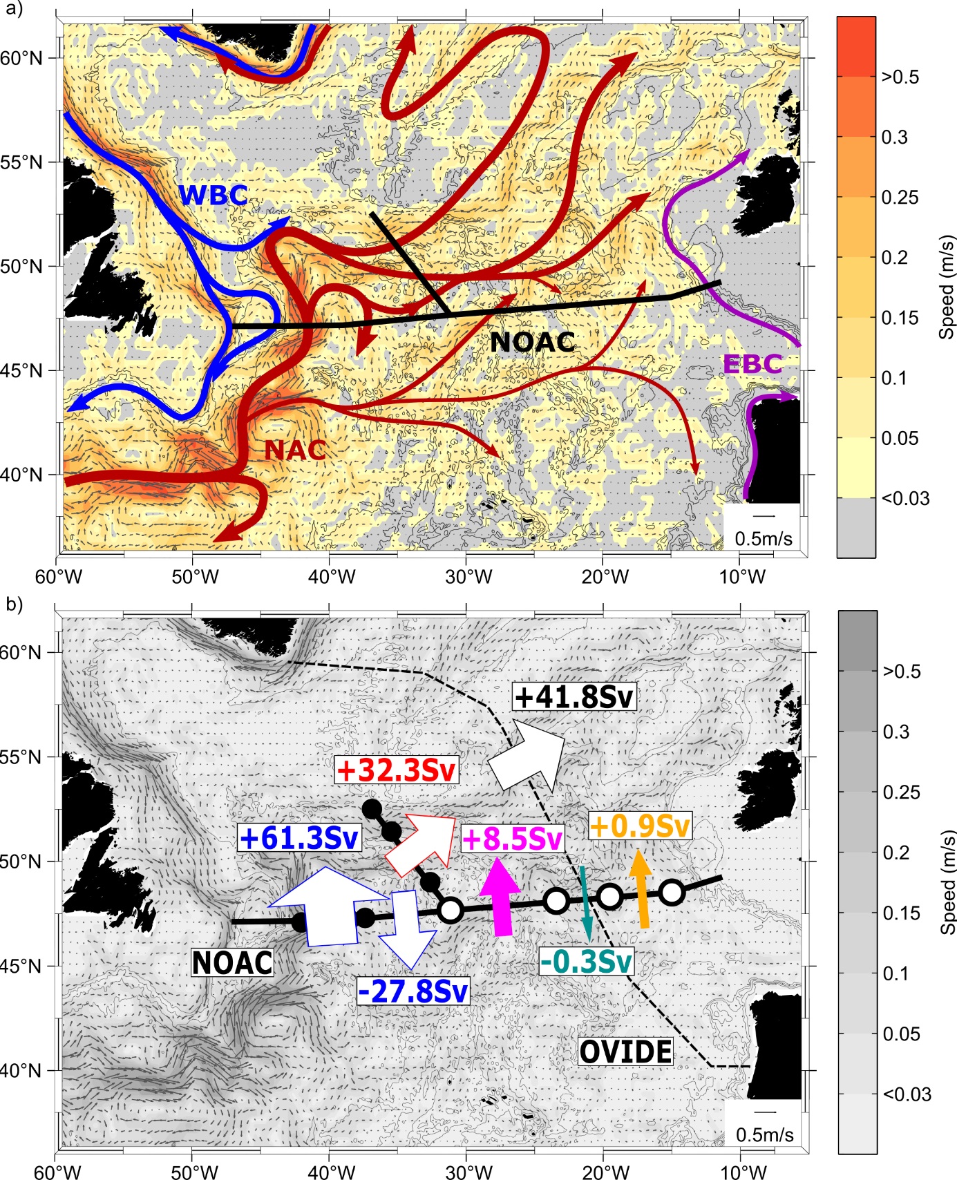
Within the North Atlantic Current, warm and salty water is transported from the subtropics into the subpolar North Atlantic. The well-studied main branch of this ocean current crosses the latitude of 47°/48°N in the western North Atlantic, turns eastward further north and crosses the Mid-Atlantic Ridge (MAR), before entering the eastern subpolar basin. By combining data from moored instruments with satellite observations, wecalculate how much water is transported north- and southward across 47°/48°N in the interior eastern basin. In addition to the well-known pathway into the subpolar eastern basin crossing the MAR further north, our data reveal a more direct pathway from the south crossing 47°/48°N in the eastern basin. This pathway contributes 22% to the total inflow into the subpolar eastern basin. The two pathways into the eastern subpolar basin are anticorrelated: the strength of the flow across the MAR decreases when the northward flow in the eastern basin across 47°/48°N increases and vice versa. Moreover, the northward flow across 47°/48°N in the interior eastern basin has increased since 1993 while the flow across 47°/48°N in the western basin has decreased.
Related projects:
IRTG ArcTrain (‘Processes and impacts of climate change in the North Atlantic Ocean and the Canadian Arctic’): https://www.marum.de/Ausbildung-Karriere/ArcTrain.html
RACE: Regional Atlantic Circulation and Global Change: https://race-synthese.de/
Further reading:
Nowitzki, H., M. Rhein, A. Roessler, D. Kieke, and C. Mertens (2021), Trends and transport variability of the circulation in the subpolar eastern North Atlantic. Journal Geophysical Research: Oceans, 126, doi:10.1029/2020JC016693.
Rhein, M., Mertens, C., and A. Roessler (2019), Observed transport decline at 47°N, Western Atlantic. Journal of Geophysical Research: Oceans, 124, doi:10.1029/2019JC014993.
Roessler, A., M. Rhein, D. Kieke, and C. Mertens (2015), Long-term observations of North Atlantic Current transport at the gateway between western and eastern Atlantic. Journal of Geophysical Research, 120, doi:10.1002/2014JC010662.
Januar 2021:
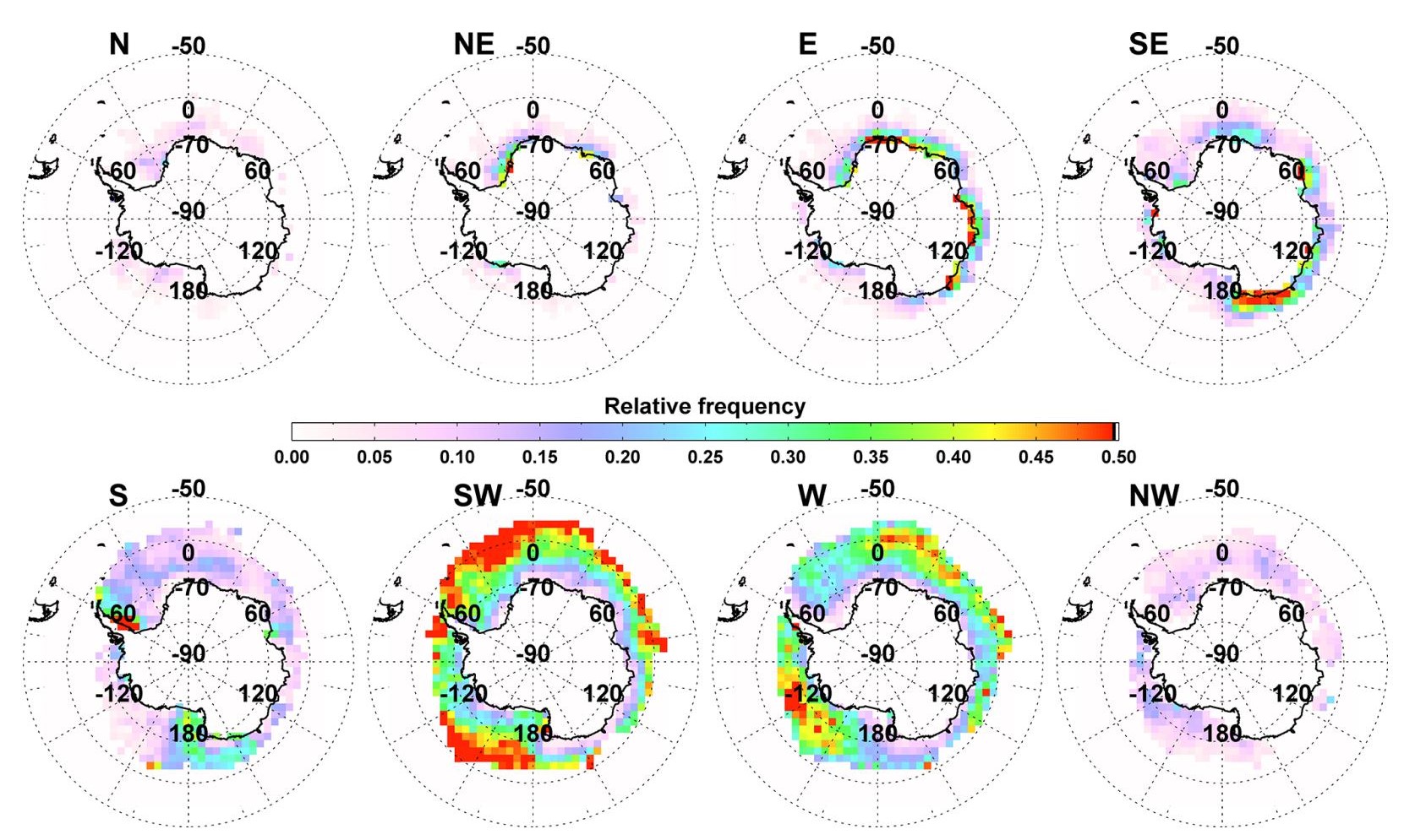
Spatial distribution of enhanced BrO and its relation to meteorological parameters
Strong enhancements of BrO concentrations in the atmospheric boundary layer are frequently observed in Polar spring in both hemispheres. They are the result of autocatalytic processes releasing bromine of maritime origin from the liquid to the gas phase. The release is driven by heterogeneous reactions thought to be taking place on the cold and saline surfaces of blowing snow, frost flowers or snow pack.
When and where exactly the BrO explosions are taking place depends not only on the availability of saline surfaces, but also to a large degree on meteorological parameters such as temperature, pressure, wind speed and direction as well as boundary layer height. Seo et al. (2020) used a time series of 10 years of GOME2 BrO retrievals to study these dependencies in both hemispheres in detail. Systematic differences were found in the meteorological conditions prevailing during BrO events when compared to mean values. In both hemispheres, low-pressure systems, cold air temperature, high surface wind speed, and a decrease of tropopause height have all higher probability during BrO events than on average. The occurrence of enhanced total BrO columns is closely associated with winds from the northwest, west, and north in the Arctic sea ice region, whereas the dominant wind direction in the Antarctic region during BrO enhancements is from the southwest and south, with systematic patterns for individual regions (see image). More details on the study can be found in Seo et al., 2020
Reference:
Seo, S., Richter, A., Blechschmidt, A.-M., Bougoudis, I., and Burrows, J. P.: Spatial distribution of enhanced BrO and its relation to meteorological parameters in Arctic and Antarctic sea ice regions, Atmos. Chem. Phys., 20, 12285–12312, https://doi.org/10.5194/acp-20-12285-2020, 2020.
Dezember 2020:

Text: Rasmus Nüß, Nikos Daskalakis, Oliver Schneising, Michael Buchwitz and Mihalis Vrekoussis
Top-down fire CO emissions optimization using TM5-4dvar and TROPOMI S5P
This study aims at optimizing the carbon monoxide (CO) emissions of the two large wildfires in Camp and Woolsey, California, that started on November 8th, 2018 and raged for multiple weeks. All the above figures show aggregated data for the main burning period of ten days (starting on the 6th is an unfortunate necessity due to model internal discretization).
To this end, the TM5-4dvarinverse model has been used to optimize the CO emissions from biomass burning provided by the Global Fire Emissions Database Version 4, including small fire boost (GFEDv4.1s) as well as the CO production from VOCs and methane on a global scale for October to December 2018. The inversion was driven by TROPOMI CO satellite observations (a) and NOAA surface flasks stations (not shown).
Figure (b) shows the modeled total column concentrations after the initial (a priori) forward run as sampled at the times and locations of the satellite observations with the satellites averaging kernel applied, i.e., what the satellite would have seen if the true atmosphere was equal to the atmosphere in the model. The mismatch between the a priori concentrations and the satellite observations (c) shows a clear overestimation over Asia and the northern hemispheric background at large. This background discrepancy could lead to an underestimation of the biomass burning source in a local inversion. Considering the relatively long lifetime of CO of about one-month, long-range transport patterns become relevant for the background. Hence a global inversion was conducted. Additionally, most of the background discrepancy can likely be attributed to an overestimation of the chemical production of CO from VOCs and methane (instead of biomass burning), which is why this source needed to be optimized simultaneously as well. It is possible to tell this source apart from the biomass burning source because changes in the former have significantly smaller temporal and spatial frequencies. Yet, some aliasing remains in the optimized emissions from both sources, which will be addressed in a later study, including additional tracers.
With this input, the model then tried in an iterative process to find the emissions that lead to concentrations as close as possible to the observations while not differing too much from the initial emissions. Figure (d) shows the resulting biomass burning emission increment, i.e., the change from the initial (a priori) to the final (a posteriori) emissions. The change in production from VOCs and methane is not pictured. In this figure, the region of interest (highlighted in the inner box, with Camp near the upper left and Woolsey in the lower right corner) is embedded in a 1° by 1° zooming region over North America. In comparison, the rest of the globe is simulated at 6° by 4° to save computational capacities. Within this region, the total emission increment over the main burning period shows only a slight increase (~12%) compared to GFED4.1s; however, most of this increment is aggregated in the pixel that contains Camp, while the adjacent pixels, all the way down to Woolsey, show small negative increments.
Running the model again with the a-posteriori emissions leads to concentrations (e) much closer to the observations. Their difference (f) is a lot closer to zero, especially in the zooming region over North America.
November 2020:
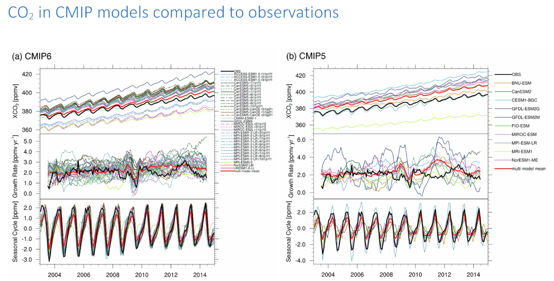
This figure (Figure 3 of Gier et al. (2020)) shows the global mean timeseries of monthly mean column-averaged dry-air mole fraction of CO2 (XCO2) for satellite observations and model data from emission driven runs of Earth System Models (ESMs) participating in the Coupled Model Intercomparison Project Phase 6 (CMIP6, Eyring et al. (2016)) and CMIP5 (Taylor et al., 2012). The models are sampled as the satellite observations (Buchwitz et al., 2018), with the panels showing the timeseries (top), the monthly growth rate (middle), and the seasonal cycle (bottom). For CMIP6 all available ensemble members, i.e. runs started from different points of the pre-industrial control simulation, are used to show the intrinsic variability of the models. The multi-model mean includes only the first ensemble member of each model, to not skew the result towards models with many ensemble members. In most cases ensemble members show a similar behavior to one another. The spread in the total value of the global mean has not been reduced by much in CMIP6 compared to CMIP5, although the multi-model mean bias has been reduced from +10ppmv to +2ppmv. The multi-model mean has a slight positive offset for the growth rate, which quantifies how fast the CO2 concentration is rising. The timeseries shows a clear seasonal cycle due to the absorption of CO2 by plants for photosynthesis in the summer, and a release of CO2 through respiration in the winter, which are both dominated by larger vegetated areas in the northern hemisphere. The CMIP6 models show a large improvement compared to CMIP5 in their ability to reproduce the seasonal cycle seen in the satellite observations.
The artifact in the growth rate in 2009 is due to the start of data coming from a second satellite, whose timeseries shows a differently shaped seasonal cycle and thus influences the growth rate due to the computation method employed here. In the annual mean growth rate this artifact is averaged out. Further sampling characteristics are discussed in Gier et al. (2020), such as the introduction of a strong negative trend in seasonal cycle amplitude with increasing XCO2 due to the spatial sampling of the satellite data. This figure was made using the Earth System Model Evaluation Tool v2 (ESMValTool, (Eyring et al., 2020; Righi et al., 2020) and will be included in the v2.2 release. The ESMValTool includes many diagnostics to use with CMIP models and observations, as well as common preprocessor functions, such as the computation of multi-model means, area averages, and the derivation of custom variables, which were used for this work. Further analysis of an updated satellite dataset is part of the Climate-Carbon Interactions in the Current Century (4C) project, which is funded by the EU under the Horizon 2020 program.
Related projects:
Advanced Earth System Model Evaluation for CMIP (Eval4CMIP)
Climate-Carbon Interactions in the Current Century (4C)
Coupled Model Intercomparison Project (CMIP)
Further reading:
Buchwitz, M., Reuter, M., Schneising, O., Noel, S., Gier, B., Bovensmann, H., Burrows, J. P., Boesch, H., Anand, J., Parker, R. J., Somkuti, P., Detmers, R. G., Hasekamp, O. P., Aben, I., Butz, A., Kuze, A., Suto, H., Yoshida, Y., Crisp, D., and O'Dell, C.: Computation and analysis of atmospheric carbon dioxide annual mean growth rates from satellite observations during 2003-2016, Atmos Chem Phys, 18, 1-22, 10.5194/acp-18-17355-2018, 2018.
Eyring, V., Bony, S., Meehl, G. A., Senior, C. A., Stevens, B., Stouffer, R. J., and Taylor, K. E.: Overview of the Coupled Model Intercomparison Project Phase 6 (CMIP6) experimental design and organization, Geosci Model Dev, 9, 1937-1958, 10.5194/gmd-9-1937-2016, 2016.
Eyring, V., Bock, L., Lauer, A., Righi, M., Schlund, M., Andela, B., Arnone, E., Bellprat, O., Brötz, B., Caron, L. P., Carvalhais, N., Cionni, I., Cortesi, N., Crezee, B., Davin, E. L., Davini, P., Debeire, K., de Mora, L., Deser, C., Docquier, D., Earnshaw, P., Ehbrecht, C., Gier, B. K., Gonzalez-Reviriego, N., Goodman, P., Hagemann, S., Hardiman, S., Hassler, B., Hunter, A., Kadow, C., Kindermann, S., Koirala, S., Koldunov, N., Lejeune, Q., Lembo, V., Lovato, T., Lucarini, V., Massonnet, F., Müller, B., Pandde, A., Pérez-Zanón, N., Phillips, A., Predoi, V., Russell, J., Sellar, A., Serva, F., Stacke, T., Swaminathan, R., Torralba, V., Vegas-Regidor, J., von Hardenberg, J., Weigel, K., and Zimmermann, K.: Earth System Model Evaluation Tool (ESMValTool) v2.0 – an extended set of large-scale diagnostics for quasi-operational and comprehensive evaluation of Earth system models in CMIP, Geosci. Model Dev., 13, 3383-3438, 10.5194/gmd-13-3383-2020, 2020.
Gier, B. K., Buchwitz, M., Reuter, M., Cox, P. M., Friedlingstein, P., and Eyring, V.: Spatially resolved evaluation of Earth system models with satellite column averaged CO2, Biogeosciences Discuss., 2020, 1-40, 10.5194/bg-2020-170, accepted, 2020.
Righi, M., Andela, B., Eyring, V., Lauer, A., Predoi, V., Schlund, M., Vegas-Regidor, J., Bock, L., Brötz, B., de Mora, L., Diblen, F., Dreyer, L., Drost, N., Earnshaw, P., Hassler, B., Koldunov, N., Little, B., Loosveldt Tomas, S., and Zimmermann, K.: Earth System Model Evaluation Tool (ESMValTool) v2.0 – technical overview, Geosci. Model Dev., 13, 1179-1199, 10.5194/gmd-13-1179-2020, 2020.
Taylor, K. E., Stouffer, R. J., and Meehl, G. A.: An Overview of CMIP5 and the Experiment Design, Bulletin of the American Meteorological Society, 93, 485-498, 10.1175/bams-d-11-00094.1, 2012.
Oktober 2020:
Record low ozone above the Arctic during spring 2020:
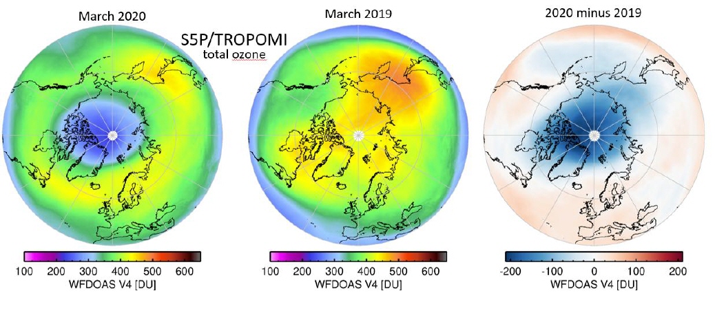
This year very low total ozone was observed in March over a large part of the Arctic. Compared to one year before total ozone levels were up to 200 DU lower this year. These low ozone levels were observed in a strong cyclone in the lower stratosphere (~20 km altitude), called the polar vortex. Temperatures inside such a cyclone are sufficiently low to form polar stratospheric clouds that activate halogens from their reservoir species and resulting in substantial chemical depletion (polar ozone loss) in late winter and early spring. Such conditions are very typical during Antarctic winter/spring (“Antarctic ozone hole”) but occur sporadically in the Arctic. A similar event in the northern hemisphere was last observed in March 2011 nine years ago. Total ozone columns regulate how much harmful UV radiation can reach the surface. We retrieved the total ozone using spectral measurements from the TROPOMI instrument aboard the Sentinel 5 Precursor satellite launched in October 2017. Our analysis showed that the minimum total ozone column north of 50°N were at a record low throughout March and April 2020. While global ozone levels are slowly recovering due to the slow decline in man-made stratospheric halogens following the phase-out of ozone-depleting substances regulated by the Montreal Protocol and Amendments, such extreme events will likely happen again, about once per decade in the future.
Mark Weber (weber@uni-bremen.de)
September 2020:
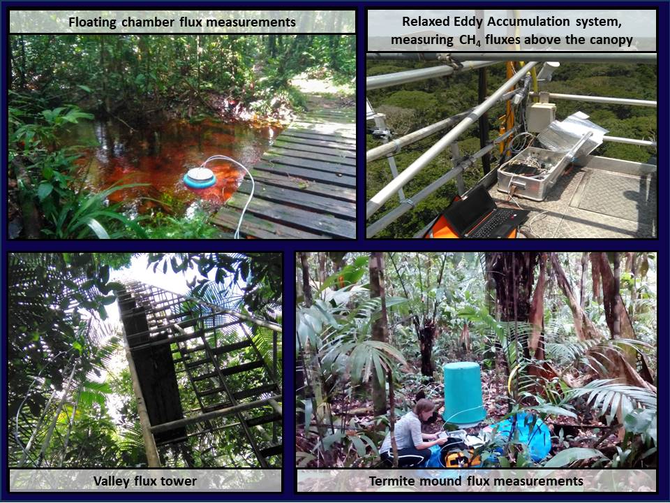
The sources and sinks of methane (CH4) in tropical rainforests are still a large source of uncertainty, and flux measurements are rare. In October 2018, INPA (National Institute for Amazonian Research, Manaus) and IUP started collaborative measurements, focusing on ecosystem CH4 flux measurements. An FTIR-analyzer, measuring CO2, CO, CH4, N2O and δ13CO2, was installed at a 50 m flux tower, measuring fluxes and concentrations of CH4. In addition, by use of a portable instrument, CH4 and CO2 flux measurements of soil, water, trees and termites were performed. Preliminary results show that the ecosystem is a small but constant source of methane, and reveal the possible large role termites play in this ecosystem.
Juni 2020:
Carbon monoxide emissions from industrial facilities
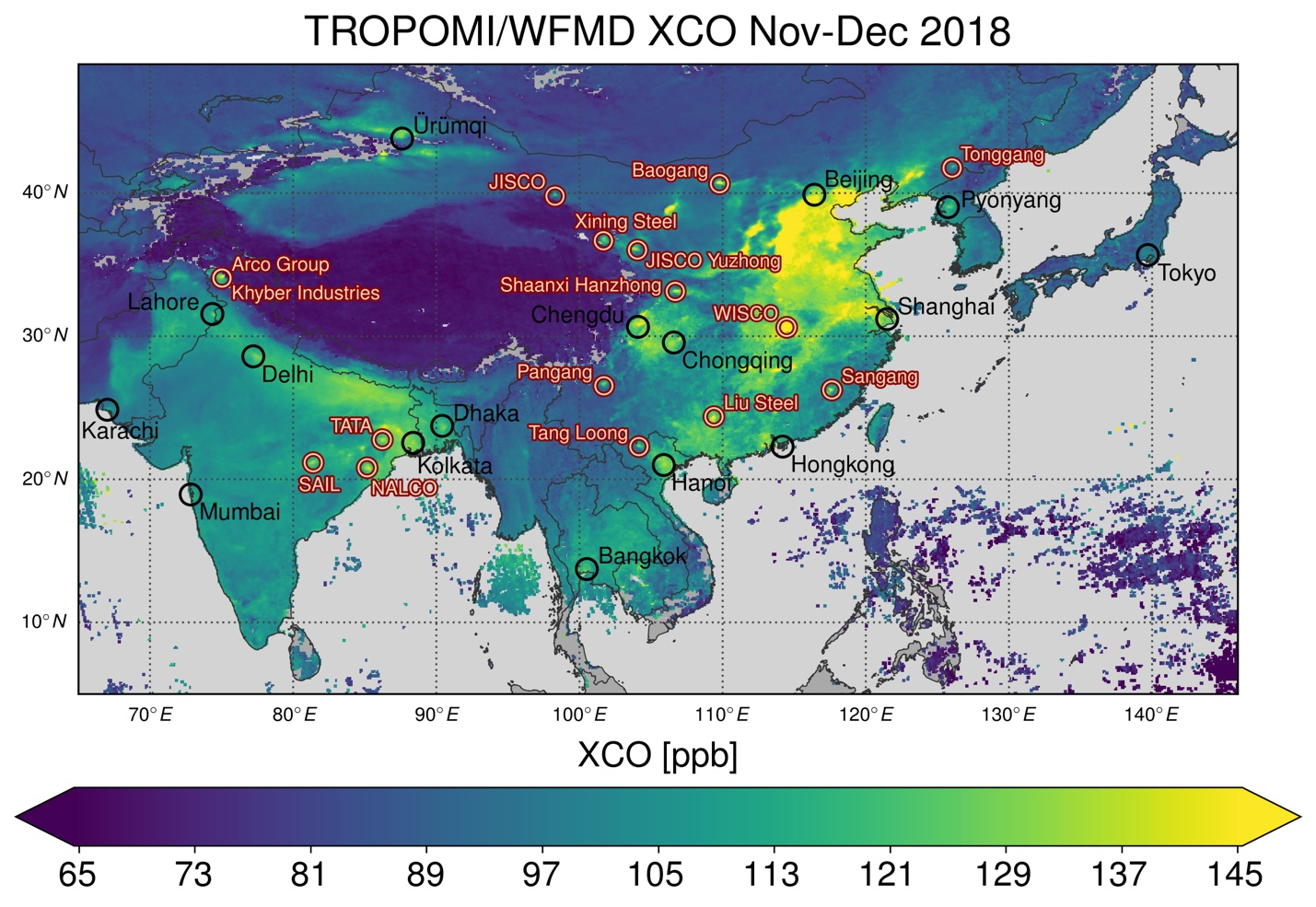
The TROPOspheric Monitoring Instrument (TROPOMI) onboard the Sentinel-5 Precursor satellite allows for the analysis of several atmospheric species, including carbon monoxide (CO) and methane (CH4), with an unprecedented level of detail by combining high precision and spatial resolution with daily global coverage.
The figure shows the CO distribution for November and December 2018 over China, India, and Southeast Asia highlighting emissions of congested urban areas and industrial facilities. The 2-month-average was chosen to get an overview of the complete region. Typically, large emission sources can even be detected in a single satellite overpass. The tracked facilities mainly belong
to the Chinese and Indian iron and steel industry. CO enhancements due to emissions from steel works are also detected in other regions of the world, for example in Turkey and Poland.
In steelmaking CO is formed during two processes. Firstly, it is an essential constituent of the blast furnace gas, which emerges when iron ore is reduced with coke to metallic pig iron. As the resulting pig iron has a relatively high carbon content, further processing is necessary to harden the metal. Therefore, the carbon-rich molten pig iron is converted to steel by lowering its carbon content via oxidation in the oxygen converter process (Linz-Donawitz-steelmaking). The resulting converter gas predominantly consists of CO.
Reference:
Schneising, O., Buchwitz, M., Reuter, M., Bovensmann, H., Burrows, J. P., Borsdorff, T., Deutscher, N. M., Feist, D. G., Griffith, D. W. T., Hase, F., Hermans, C., Iraci, L. T., Kivi, R., Landgraf, J., Morino, I., Notholt, J., Petri, C., Pollard, D. F., Roche, S., Shiomi, K., Strong, K., Sussmann, R., Velazco, V. A., Warneke, T., and Wunch, D.: A scientific algorithm to simultaneously retrieve carbon monoxide and methane from TROPOMI onboard Sentinel-5 Precursor, Atmos. Meas. Tech., 12, 6771–6802, https://doi.org/10.5194/amt-12-6771-2019, 2019.
April 2020:
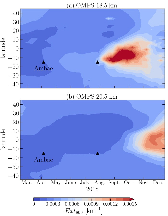
Stratospheric aerosols are an essential component of the climate system. Firstly, they change the radiative budget of the Earth, and secondly, they play an important role in ozone depletion. There is a background stratospheric aerosol layer build by the sulfuric gas emissions from the ocean surface; however, this layer is occasionally perturbed by volcanic eruptions which emit aerosol precursors directly in the stratosphere.
In the figure above, the changes in stratospheric aerosol loading after the 2018 eruption of Ambae are shown. Ambae, a volcanic island in South Pacific (Vanuatu), continuously erupted for over a year in 2017-2018; and it was the strongest volcanic eruption in the world for those two years. There were two eruption episodes when sulfuric gases reached the stratosphere, namely, on April 6 and on July 28, 2018. In the figure above, 10-day averaged aerosol extinction coefficient at 869 nm retrieved from OMPS-LP data is presented at 18.5 km (panel (a)) and at 20.5 km (panel (b)) as a function of latitude and time. The location and time of the eruption are marked by the black triangles. There is a slight increase in the aerosol extinction coefficient at 18.5 km after the fist, smaller eruption. At the same time, the increase after the second eruption is much larger; this is because the triple amount of precursor gases was emitted during the July episode. For both eruptions, the increase becomes noticeable right after the precursors were emitted, but the plume intensifies in about a month. This corresponds to the time needed for oxidation of the precursors to aerosols.
In particular after the second eruption, aerosols are not only localized in the tropics and are transported in the higher latitudes. Thus, the volcanic impact is seen at 18.5 km at 45°, both North and South, in late December 2018. In the tropics, at that time, the plume starts to dissipate; however, it still does not vanish completely. Such distribution of a volcanic plume is typical for a tropical eruption, as the Brewer-Dobson circulation moves the stratospheric air masses polewards from the equator.
Another resulting pattern of the Brewer-Dobson is aerosol distribution at 20.5 km. There, the increase after the first eruption is rather small; it appears in mid-May and lasts until the second eruption. The delay by approximately 1.5 months in the extinction increase at the higher altitudes is caused by convection. The lofting air in the tropics transports the aerosols and their precursors upwards. The time lag until the perturbation reaches higher altitudes is often referred to as a tape-recorder effect. After the second eruption, the plume appears at 20.5 km with 6-7 weeks delay as well. At this altitude, the maximal extension of the volcanic plume is achieved in November-December 2018. At the very end of 2018, the aerosols are transported to the higher latitudes, and the plume starts to dissipate.
This study shows the global impact of tropical volcanic eruptions. Even though their radiative forcing might be lower than for the extratropical eruptions of the same magnitude, the effect is seen all over the globe and does not stick to a particular location.
Reference: Malinina, E., Rozanov, A., Niemeier, U., Peglow, S., Arosio, C., Wrana, F., Timmreck, C., von Savigny, C. and Burrows, J. P. : Changes in stratospheric aerosol extinction coefficient after the 2018 Ambae eruption as seen by OMPS-LP and ECHAM-HAM, to be submitted in ACP in May 2020.
März 2020:
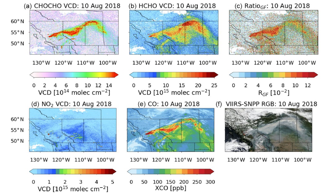
Wild fires are known to emit large quantities of trace gases and aerosols into the atmosphere, resulting in air pollution in the vicinity of the fires but often also at long distances downwind of the fires. In August 2018, unusually high temperatures caused severe drought in some areas of North America and resulted in the outbreak of many wildfires: the province of British Columbia (BC) in Canada was one of the most affected areas. Some of these fires were large enough to create enough heat to lift the emissions into the free troposphere where they were transported over long distances.
Measurements of the TROPOMI instrument on the European Sentinel 5 precursor satellite can be used to retrieve the column amounts of several trace gases emitted by wild fires (see figure). On August 10, 2018, a huge plume of particles and gases emitted from several big fires was covering large parts of North America, extending more than 1500 km from the location of the fires. While long-range transport of carbon monoxide (CO) has already been observed on many occasions, long-range transport of short-lived volatile organic compounds (VOCs) such as formaldehyde (HCHO) and glyoxal (CHO.CHO) is not expected as transport times are longer than the atmospheric residence time of these gases. However, the measurements show that also HCHO and CHO.CHO are present in the plume for at least a day, and comparison with FLEXPART transport modelling indicates effective lifetimes of the order of 30 hours. These unexpected observations are best explained by continuous production of HCHO and CHO.CHO from long-lived precursors in the plume, the nature of which still needs to be investigated.
This study highlights the importance of wild fires for air quality both locally and at a distance, an important aspect in a changing climate where hot and dry years such as 2018 are expected to become more frequent, resulting in more and bigger fires. It also demonstrates the power of S5P satellite observations which provide global trace gas column maps with high spatial resolution.
Reference:
Alvarado, L. M. A., Richter, A., Vrekoussis, M., Hilboll, A., Kalisz Hedegaard, A. B., Schneising, O., and Burrows, J. P.: Unexpected long-range transport of glyoxal and formaldehyde observed from the Copernicus Sentinel-5 Precursor satellite during the 2018 Canadian wildfires, , 20, 2057–2072, https://doi.org/10.5194/acp-20-2057-2020, 2020.
Februar 2020:
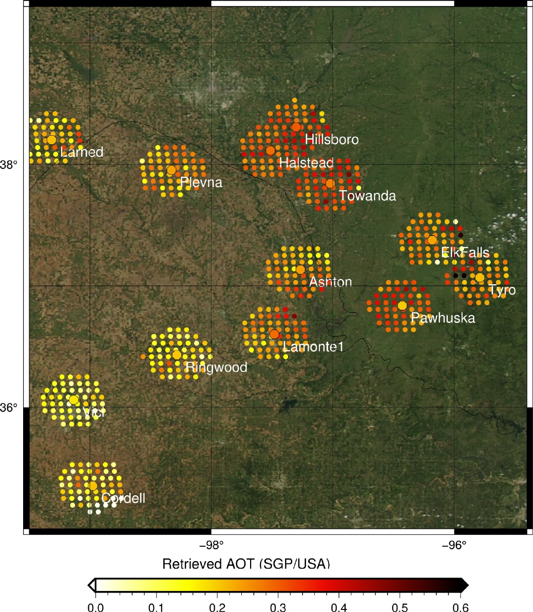
Recent work at the Institute of Environmental Physics exploits the potential of the satellite instrument POLDER which was using multi-spectral and multi-viewing capabilities, for the retrieval of suspended liquid or solid particles in air (also known as aerosols), as well as surface properties.
The image shows the Aerosol Optical Depth (AOT) which is ia important parameter describing the overall atmospheric aerosol burden. The study aims at retrieving AOT and surface reflectance at high quality which are important quantities for the modeling community as well as crucial parameters for air quality assessment from space. The agreement of the first results with ground-based measurements, as shown in the figure is very promissing: the color-coded points at the center of each station are close to the retrieved values based on satellite data.
This is of particular relevance because within the next decade a fleet of upcoming satellite instruments will provide measurements similar to POLDER which can be evaluated with the newly developed methodology.
Reference: Marco Vountas, Kristina Belinska, Vladimir V. Rozanov, Luca Lelli, Linlu Mei, Soheila Jafariserajehlou, John P. Burrows, "Retrieval of aerosol optical thickness and surfaceparameters based on multi-spectral and multi-viewing space-borne measurements" (2020).