Image of the Month

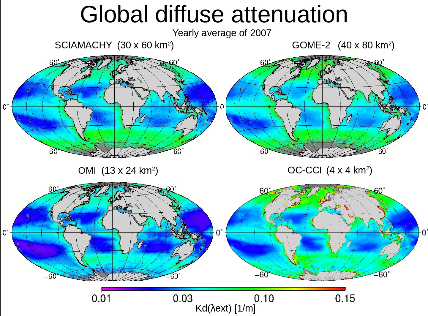
Average global distribution of diffuse attenuation coefficient at the excitation wavelength region 390 to 426 nm (Kd(λext)) from Feb until Dec 2007. The diffuse attenuation coefficient is a measure of how deep the sunlight penetrates the ocean. It helps characterizing the underwater light field which is important for estimating the heat budget and primary production in the global oceans. The diffuse attenuation coefficient was derived from three atmospheric satellite sensors SCIAMACHY, GOME-2, and OMI by retrieving vibrational Raman scattering fit factors using Differential Optical Absorption Spectroscopy and converting these to Kd(λext) via Look-up-Tables based on radiative transfer modeling. The standard diffuse attenuation product OC-CCI (Kd490) as obtained from multispectral ocean color satellites was converted to the excitation wavelength region and is shown in comparison. Figure adapted from Oelker et al. (2019).

Recent work at the Institute of Environmental Physics exploits the potential of TROPOMI for ocean applications in a project funded by ESA and led by the Alfred-Wegener-Institute in Bremerhaven (S5POC, https://eo4society.esa.int/projects/sentinel-5pinnovation/). TROPOMI is a satellite sensor on board Sentinel-5P, a recent atmospheric satellite mission launched in October 2017 dedicated for detecting atmospheric trace gases such as ozone and nitrogen dioxide. The possibility to derive diffuse attenuation in the blue and additionally in the ultraviolet region ofthe solar spectrum, as well as the quantification of different phytoplankton groups and the fluorescence signal of phytoplankton will be explored.

Reference: Julia Oelker, Andreas Richter, Tilman Dinter, Vladimir V. Rozanov, John P. Burrows, and Astrid Bracher, "Global diffuse attenuation derived from vibrational Raman scattering detected in hyperspectral backscattered satellite spectra," Opt. Express 27, A829-A855 (2019).

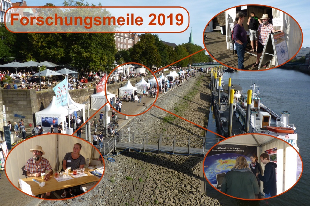
Forschungsmeile 2019

On 21 and 22 September IUP participated again at the ‘Forschungsmeile’ during the ‘Maritime Woche 2019’ in Bremen. In a small tent close to the Weser at the ‘Schlachte’ the working groups Physics and Chemistry of the Atmosphere and Remote Sensing presented highlights of their current research areas to the public, especially related to observations of sea ice, air quality and greenhouse gases from satellites. In addition to the famous ‘ice cube experiment’ (Does an ice cube melt faster in fresh water or seawater?) visitors could measure on-site CO2 and methane concentrations of their breath. The nice weather brought a lot of interested people to the Schlachte, such that the event is considered successful by all participants.

Contact: Stefan Noël (stefan.noel@iup.physik.uni-bremen.de)

The September picture of the month shows the modelling of methane dispersion using FLEXPART-WRF.

Methane is an important greenhouse gas. Getting extended knowledge about the sinks and sources is therefore an important task. Modelling the transport of emissions can help a) to plan future measurement campaigns and, b) in combination with measurements, to validate the given emission estimates.

The Upper Silesian Coal Basin is a coal basin in Silesia (Poland, Czech Republic). It contains numerous mines exploiting its large coal reservoirs. When the coal is extracted from the earth, considerable amounts of methane are released, which is extracted from the underground mines and released into the atmosphere through venting shafts. The methane emitted from the Upper Silesian Coal Basin constitutes a regionally significant source.

The fact that the emission takes place at a limited number of well-known locations allows for detailed simulation of the dispersion of the emitted methane in the atmosphere. The latter, combined with measurements of the atmospheric methane concentration,can yield important insight into the emitted quantities.

FLEXPART-WRF is a Lagrangian atmospheric transport model which uses meteorological data (e.g., wind fields) from simulations using the Weather Research and Forecast model WRF. Practically, this means that it allows the simulation of atmospheric transport processes at very small spatial scales of on the order of ~100m.

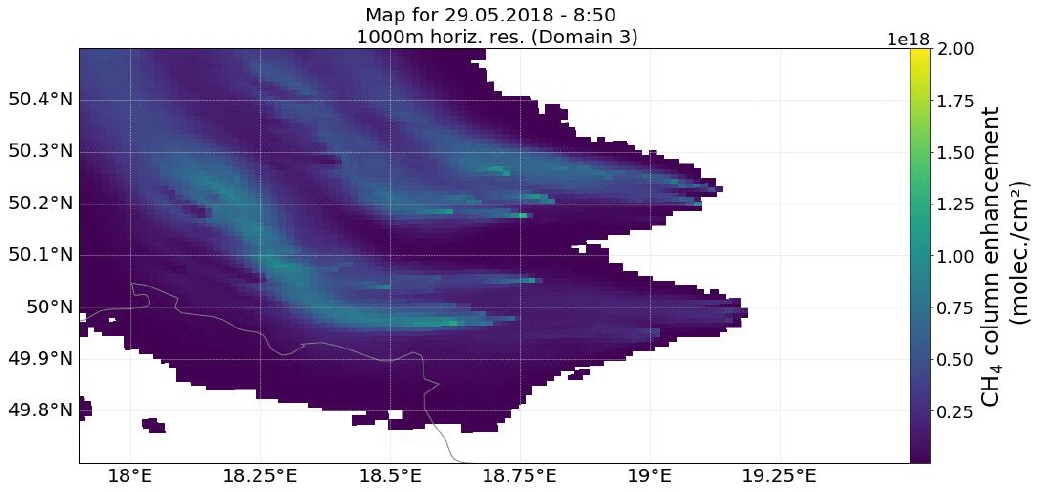
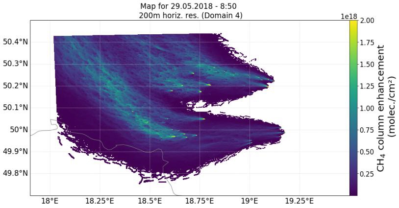
Figures a) – b) show the simulated methane column enhancement (i.e., ignoring the high methane background of the atmosphere) emitted in Upper Silesia on the morning of 29 May 2018. For Image a) wind fields at a spatial resolution of 1km per grid box were used while b) uses wind fields ata spatial resolution of 200m.

One can see considerably finer structured plumes when using the higher spatial resolution. Even if the general shape of the plumes is comparable in both figures, when taking a closer look one can see that at 1km resolution, the detailed shape of the plume is different (it starts turning northwards earlier, i.e., closer to the emission sources, at 200m resolution).

These high-resolution simulations allow better analysis of methane measurements executed by the airborne MaMap instrument during the CoMet campaign in spring 2018 (ongoing work)

Acknowledgements: All simulations were conducted on the Aether HPC cluster at University of Bremen, financed by DFG within the scope of the Excellence Initiative.

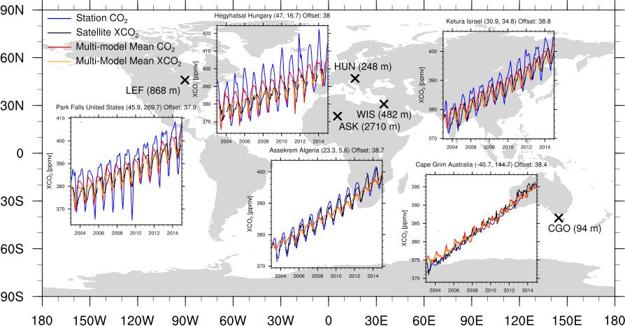
The figure shows the time series of CO2 and XCO2 (column-averaged dry-air mole fraction of CO2) for satellite observations, station data, and the mean calculated from emission driven runs of two Earth System Models (ESMs) participating in the Coupled Model Intercomparison Project Phase 6 (CMIP6) (Eyring et al. 2016a) for the years 2003-2014. The satellite observations (Buchwitz et al. 2018) combine measurements of SCIAMACHY (SCanning Imaging Absorption Spectrometer for Atmospheric CHartographY) on Envisat and TANSO-FTS (Thermal And Near infrared Sensor for carbon Observation - Fourier Transform Spectrometer) on GOSAT (Greenhouse gases Observing SATellite). The station data are from the NOAA/ESRL (National Oceanic and Atmospheric Administration/Earth System Research Laboratory) surface measurements.

All data are processed using the Earth System Model Evaluation Tool (ESMValTool, Eyring et al. (2016c)). Currently, a release of a new version (v2.0) of the ESMValTool is in preparation, which is developed to analyze CMIP6 model simulations as soon as they are published to the CMIP6 archive. It includes a large collection of diagnostics and performance metrics for atmospheric, oceanic, and terrestrial variables for the mean state, trends, and variability. Here, the ESMValTool is used to convert the model results to XCO2, the quantity provided from satellite measurements, and for the sampling of the models in the same way than the observations. For better comparison of the seasonal cycle, the models results are corrected for an offset to the satellite data.

Models and observations show the expected increase in CO2and the characteristic seasonal cycles most pronounced in the Northern Hemisphere, with lower values in the summer when strong photosynthesis causes plants to absorb CO2, and higher values in the winter when photosynthesis stops and CO2is released through respiration. The amplitude of the seasonal cycle differs between models and observations. The reason for this difference and potential future changes will be further evaluated within the Advanced Earth System Model Evaluation for CMIP (EVal4CMIP) project funded by the Helmholtz Society. Changes in the seasonal cycle are expected because of the CO2 fertilization effect (Wenzel et al. 2016). New emergent constraints (Eyring et al. 2019) for the carbon-climate and CO2 fertilization effects are going to be developed within the “Climate-Carbon Interactions in the Coming Century” (CCiCC) project that is funded by the EU under the Horizon 2020 program. Further research within CCiCC includes the analysis of new data sets and recommendations for model improvements and observational strategies.

Related projects:

Advanced Earth System Model Evaluation for CMIP (EVal4CMIP)

Climate-Carbon Interactions in the Coming Century (CCiCC)

Coupled Model Intercomparison Project (CMIP)

Further reading:

Buchwitz, M., Reuter, M., Schneising, O., Noel, S., Gier, B., Bovensmann, H., Burrows, J.P., Boesch, H., Anand, J., Parker, R.J., Somkuti, P., Detmers, R.G., Hasekamp, O.P., Aben, I., Butz, A., Kuze, A., Suto, H., Yoshida, Y., Crisp, D., & O'Dell, C. (2018). Computation and analysis of atmospheric carbon dioxide annual mean growth rates from satellite observations during 2003-2016. Atmospheric Chemistry and Physics, 18

Eyring, V., Bony, S., Meehl, G.A., Senior, C.A., Stevens, B., Stouffer, R.J., & Taylor, K.E. (2016a). Overview of the Coupled Model Intercomparison Project Phase 6 (CMIP6) experimental design and organization. Geoscientific Model Development, 9, 1937-1958

Eyring, V., Cox, P.M., Flato, G.M., Gleckler, P.J., Abramowitz, G., Caldwell, P., Collins, W.D., Gier, B.K., Hall, A.D., Hoffman, F.M., Hurtt, G.C., Jahn, A., Jones, C.D., Klein, S.A., Krasting, J.P., Kwiatkowski, L., Lorenz, R., Maloney, E., Meehl, G.A., Pendergrass, A.G., Pincus, R., Ruane, A.C., Russell, J.L., Sanderson, B.M., Santer, B.D., Sherwood, S.C., Simpson, I.R., Stouffer, R.J., & Williamson, M.S. (2019). Taking climate model evaluation to the next level. Nature Climate Change, 9, 102-110

Eyring, V., Gleckler, P.J., Heinze, C., Stouffer, R.J., Taylor, K.E., Balaji, V., Guilyardi, E., Joussaume, S., Kindermann, S., Lawrence, B.N., Meehl, G.A., Righi, M., & Williams, D.N. (2016b). Towards improved and more routine Earth system model evaluation in CMIP. Earth System Dynamics, 7, 813-830

Eyring, V., Righi, M., Lauer, A., Evaldsson, M., Wenzel, S., Jones, C., Anav, A., Andrews, O., Cionni, I., Davin, E.L., Deser, C., Ehbrecht, C., Friedlingstein, P., Gleckler, P., Gottschaldt, K.D., Hagemann, S., Juckes, M., Kindermann, S., Krasting, J., Kunert, D., Levine, R., Loew, A., Makela, J., Martin, G., Mason, E., Phillips, A.S., Read, S., Rio, C., Roehrig, R., Senftleben, D., Sterl, A., van Ulft, L.H., Walton, J., Wang, S.Y., & Williams, K.D. (2016c). ESMValTool (v1.0) - a community diagnostic and performance metrics tool for routine evaluation of Earth system models in CMIP. Geoscientific Model Development, 9, 1747-1802

Wenzel, S., Cox, P.M., Eyring, V., & Friedlingstein, P. (2016). Projected land photosynthesis constrained by changes in the seasonal cycle of atmospheric CO2. Nature, 538, 499-501

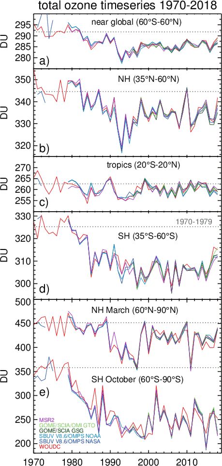
Midlatitude total ozone means were high in 2018, while the tropical values were low compared to the annual means observed in the recent decade as seen in Fig. 1, which shows the annual mean total ozone time series from various merged datasets (five satellite datasets and one based upon groundbased instruments) for the near-global (60°N–60°S) average, tropics, extratropics, and selected months in the polar regions.

For all latitude bands, except the tropics, the average total ozone levels have not yet recovered to the values of the 1970s, a time when ozone losses due to ozone-depleting substances (ODSs) were still very small (WMO 2018). Total ozone is defined as the vertical column amount or in other words the number of ozone molecules above a unit area. Typical units are Dobson units (DU) and the global average column amount is about 300 DU. The lower the ozone column, the higher is the amount of harmful UV radiation reaching the surface that can damage plant cells as well as cause skin cancer.

A recent study by us (Weber et al. 2018a) indicates that total ozone trends since the late 1990s are positive (<1% decade−1) but at most latitudes the trends do not reach statistical significance. Still, the small increase in global total ozone following the significant decline before the 1990s provides proof that the Montreal Protocol and its later Amendments, responsible for phasing out ozone-depleting substances, has been successful. The observed changes in total ozone are reproduced well by state-of-the-art chemistry-transport model calculations that account for changes in transport and for changes in the ozone-depleting substances regulated by the Montreal Protocol (Chipperfield et al. 2018).

In Figure 1 one of the satellite merged data were produced in our institute (GSG dataset) that combines various European sensors (GOME, SCIAMACHY, GOME-2A) that were retrieved with the WFDOAS (weighting function differential absorption spectroscopy) retrievals (Coldewey-Egbers et al., 2005). The European time series started in 1995 and in 2017 and 2018 two new sensors were launched, TROPOMI and GOME-2C, respectively. Both instruments will continue long-term ozone monitoring. In particular TROPOMI provides measurements at an unprecedented spatial resolution corresponding to a foot print of 3.5 km by 7 km at the surface.

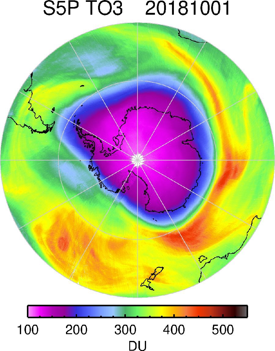
Figure 2 shows the total ozone distribution above Antarctica from 1stOctober 2018. In early October the ozone hole reaches its largest extent. In 2018 the size of the ozone hole (defined by values below 220 DU) was higher than the average from recent years. However, the extent of the ozone hole varies from year-to-year depending on the polar meteorology (colder stratospheric winters produce larger ozone holes) as seen in panel e of Fig. 1. Nevertheless, there are signs that spring time total ozone above Antarctica is beginning to recover (Weber et al., 2018, WMO 2018).


References:

Chipperfield, M. P., Dhomse, S., Hossaini, R., Feng, W., Santee, M. L., Weber, M., Burrows, J. P., Wild, J. D., Loyola, D., Coldewey-Egbers, M, 2018: On the Cause of Recent Variations in Lower Stratospheric Ozone. Geophys. Res. Lett., 45, 5718-5726, https://doi.org/10.1029/2018GL078071.

Coldewey-Egbers, M., M. Weber, L. N. Lamsal, R. de Beek, M. Buchwitz, J. P. Burrows, 2005: Total ozone retrieval from GOME UV spectral data using the weighting function DOAS approach.Atmos. Chem. Phys. 5, 5015-5025, https://doi.org/10.5194/acp-5-1015-2005.

Weber, M., Coldewey-Egbers, M., Fioletov, V. E., Frith, S. M., Wild, J. D., Burrows, J. P., Long, C.
S., and Loyola, D., 2018a: Total ozone trends from 1979 to 2016 derived from five merged
observational datasets – the emergence into ozone recovery. Atmos. Chem. Phys., 18, 2097-2117,
https://doi.org/10.5194/acp-18-2097-2018.

Weber, M., Steinbrecht, W., van der A, R., Frith, S. M., Anderson, J., Coldewey-Egbers, M., Davis, S,
Degenstein, D., Fioletov, V., Froidevaux, L., Hubert, D., de Laat, J., Long, C. S., Loyola, D., Sofieva,
V., Tourpali, K., Roth, C., Wang, R., and Wild, J.D., 2018b: Stratospheric ozone [in "State of the
Climate in 2017"], Bull. Amer. Meteor. Soc., 99, S51-S54,
https://doi.org/10.1175/2018BAMSStateoftheClimate.1.

WMO, 2018: World Meteorological Organization/United Nations of Environmental Protection,
Scientific assessment of ozone depletion, 2018. Global Ozone Research and Monitoring Project–
Report No. 58, Geneva, Switzerland, available at https://www.esrl.noaa.gov/csd/assessments/ozone/.

The extent of the sea ice around Antarctica has a marked seasonal cycle; the maximum is usually reached around September (at the end of austral winter), and the minimum in late February (at the end of austral summer). This year's minimum was reached in the last week of February. According to the sea ice data produced at IUP from satellite data (microwave radiometer AMSR2 on the Japanese satellite GCOM-W2), the lowest daily sea ice extent was 2.54 million km2 on February 23, 2019. By extent we mean the total area of all satellite pixels covered by at least 15% of sea ice.

The largest portion of remaining sea ice is, as usual, sitting in the Weddell Sea, where it is pushed towards the Antarctic Peninsula by the Weddell Gyre (middle figure). This can be compared with last year's ice extent maximum on 30 September 2018 (upper figure). The amplitude of the seasonal cycle in ice extent is more than 15 million km2, i.e. 1.5 times the size of Europe.Comparison with the other Antarctic sea ice minima since the beginning of satellite observations in 1978 (lower figure) shows that this year's minimum is low but not unique – the absolute minimum on record was in 2017. However, after an overall increase in Antarctic sea ice extent until about 2013 the last years show a strong decrease in both summer and winter.

Publications:

Spreen, G., L. Kaleschke, and G.Heygster (2008), Sea ice remote sensing using AMSR-E 89 GHz channels ,vol. 113, C02S03, doi:10.1029/2005JC003384.

AMSR2 ASI sea ice concentration data, Antarctic, version 5.4 (NetCDF) (July 2012 - December 2018). , https://doi.pangaea.de/10.1594/PANGAEA.898400


Projects:

Sea ice type distribution in the Antarctic from microwave satellite observations (SITAnt), (https://seaice.uni-bremen.de/sitant/)

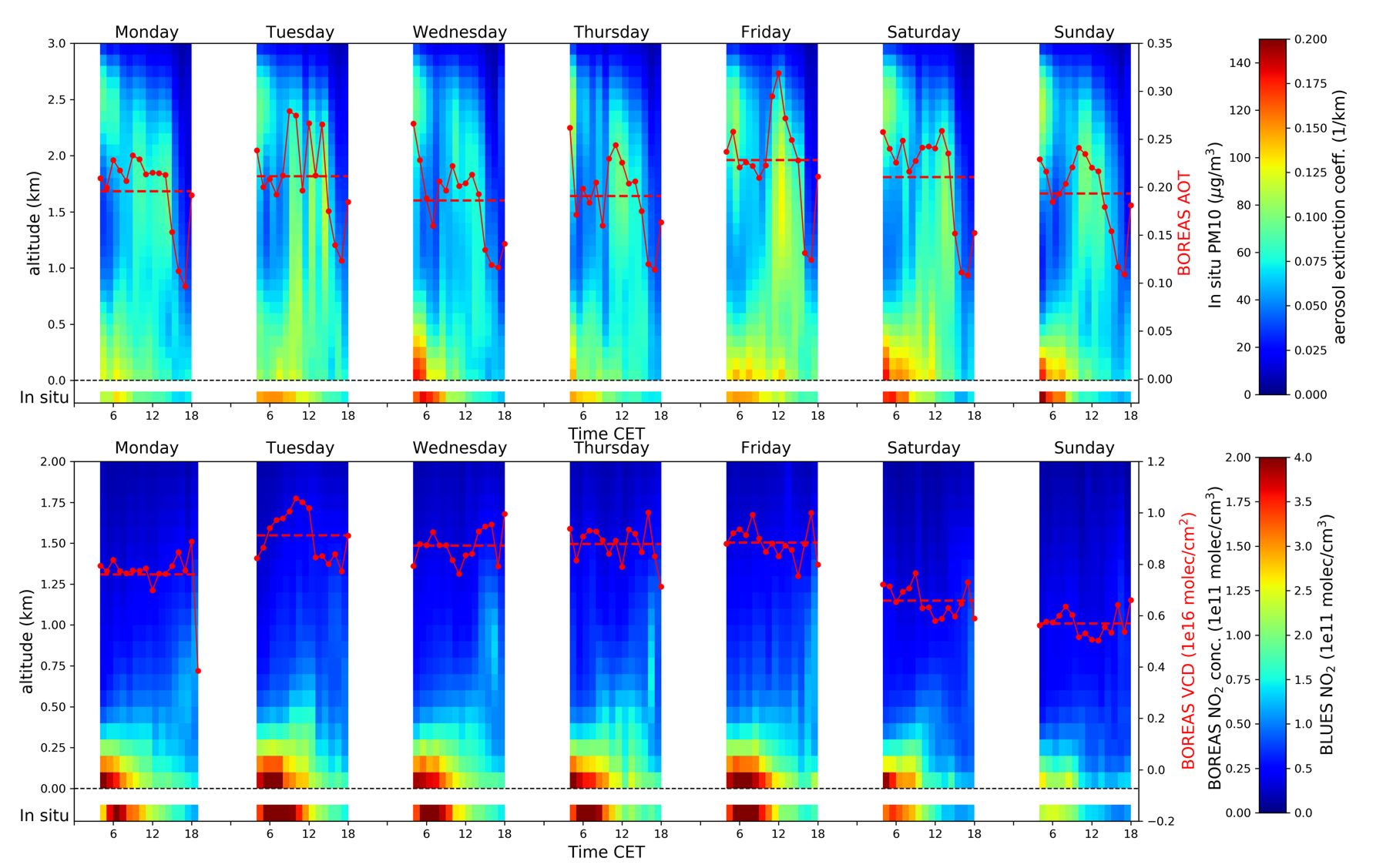
Ground based Multi-Axis Differential Optical Absorption Spectroscopy (MAX-DOAS) observations are a frequently used method to determine atmospheric column amounts of reactive gases such as ozone, nitrogen dioxide or formaldehyde. By probing the atmosphere at different elevation angles, information on the vertical distribution of these absorbers can be determined, as well as on aerosol extinction. In order to extract the profile information from the observations taken at different elevation angles, inversion algorithms are needed which combine a priori information with the information from the measurements.

The Bremen Optimal estimation REtrieval for Aerosols and trace gaseS (BOREAS) is a new, flexible profiling algorithm which combines a non-linear aerosol retrieval module with a trace gas retrieval part. Both Optimal Estimation and Levenberg Marquardt approaches are implemented, and many options for a priori selection and pre-scaling, smoothing constraints, and retrieval modes are implemented. Results from BOREAS have been compared to those from other state of the art retrievals in an extensive study using synthetic data (Frieß et al., 2018) and using measurements during the CINDI-2 campaign (Tirpitz et al., manuscript in preparation) demonstrating the good performance of the algorithm. More details on BOREAS and its validation can be found in Bösch et al., 2018.

References:

Bösch, T., Rozanov, V., Richter, A., Peters, E., Rozanov, A., Wittrock, F., Merlaud, A., Lampel, J., Schmitt, S., de Haij, M., Berkhout, S., Henzing, B., Apituley, A., den Hoed, M., Vonk, J., Tiefengraber, M., Müller, M., and Burrows, J. P.: BOREAS – a new MAX-DOAS profile retrieval algorithm for aerosols and trace gases, Atmos. Meas. Tech., 11, 6833-6859, https://doi.org/10.5194/amt-11-6833-2018, 2018.

Frieß, U., Beirle, S., Alvarado Bonilla, L., Bösch, T., Friedrich, M. M., Hendrick, F., Piters, A., Richter, A., van Roozendael, M., Rozanov, V. V., Spinei, E., Tirpitz, J.-L., Vlemmix, T., Wagner, T., and Wang, Y.: Intercomparison of MAX-DOAS Vertical Profile Retrieval Algorithms: Studies using Synthetic Data, Atmos. Meach. Teech. Discuss., https://doi.org/10.5194/amt-2018-423, in review, 2018.

BLUES - Das Bremer Luftüberwachungssystem https://www.bauumwelt.bremen.de/umwelt/luft/luftqualitaet-24505

First estimate of the CO2 year 2018 growth rate from satellites

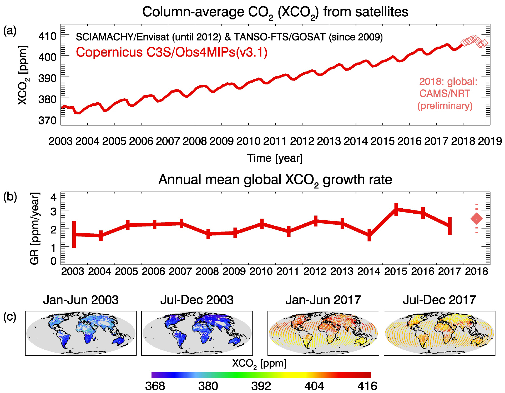
Carbon dioxide (CO2) is an important greenhouse gas and increasing atmospheric concentrations lead to global warming. The IUP of the University of Bremen develops methods to measure the atmospheric CO2distribution from space.

The picture shows in (a) time series of the vertically averaged CO2mixing ratio (“XCO2”) including preliminary values for 2018. One can see that CO2increases approximately linearly with time. This is primarily due to burning of fossil fuels. The seasonal fluctuations are primarily due to uptake and release by vegetation. The time series have been computed from satellite data, which also show the spatial distribution (see maps in (c)). The XCO2unit is ppm (parts per million). 400 ppm means that the atmosphere contains on average 400 CO2molecules per one million air molecules.

In (c) the annual mean XCO2 growth rate is shown. As can be seen, the growth rate varies somewhat from year to year. A reason for this are fluctuations of the natural CO2 sinks (e.g., forests) or increasing emissions including emissions from wildfires. The preliminary estimate of the growth rate for 2018 is 2.5 ppm/year (uncertainty range +/- 0.8 ppm/year). This is somewhat less than in 2015 and 2016 (two years with weaker than average sinks and significant wildfires partly due to the natural climate phenomenon El Niῆo) but somewhat less than 2017. Future refined analysis will show to what extent this preliminary estimate is confirmed.

Press:

Copernicus (7-Jan-2019): Press release: “Last four years have been the warmest on record – and CO2continues to rise” URL: https://climate.copernicus.eu/last-four-years-have-been-warmest-record-and-co2-continues-rise

EuroNews (14-Dec-2018): Video: “Temperatures in November above average” URL: https://www.euronews.com/2018/12/14/temperatures-in-november-above-average

Publications:

Buchwitz, M., Reuter, M., Schneising, O., Noel, S., Gier, B., Bovensmann, H., Burrows, J. P., Boesch, H., Anand, J., Parker, R. J., Somkuti, P., Detmers, R. G., Hasekamp, O. P., Aben, I., Butz, A., Kuze, A., Suto, H., Yoshida, Y., Crisp, D., and O'Dell, C., Computation and analysis of atmospheric carbon dioxide annual mean growth rates from satellite observations during 2003-2016, Atmos. Chem. Phys., 18, 17355-17370, https://doi.org/10.5194/acp-18-17355-2018, 2018. URL: https://www.atmos-chem-phys.net/18/17355/2018/

Heymann, J., M. Reuter, M. Buchwitz, O. Schneising, H. Bovensmann, J. P. Burrows, S. Massart, J. W. Kaiser, D. Crisp, CO2emission of Indonesian fires in 2015 estimated from satellite-derived atmospheric CO2concentrations, Geophys. Res. Lett., DOI: 10.1002/2016GL072042, pp. 18, 2017. URL: http://onlinelibrary.wiley.com/doi/10.1002/2016GL072042/full

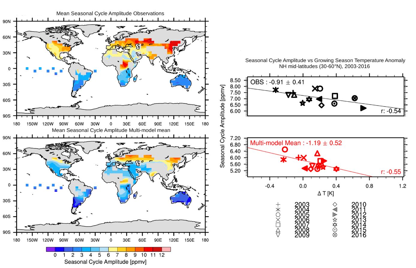
The left side of the figure shows the mean seasonal cycle amplitude of column-averaged dry-air mole fraction of CO2(XCO2) for satellite observations and the multi-model mean calculated from 10 Earth System Models (ESMs) participating in the Coupled Model Intercomparison Project Phase 5 (CMIP5) for the years 2003-2016. The models are sampled the same way as the observations. The observations (Buchwitz et al., 2018) combine measurements of SCIAMACHY (SCanning Imaging Absorption Spectrometer for Atmospheric CHartographY) on Envisat and TANSO-FTS (Thermal And Near infrared Sensor for carbon Observation - Fourier Transform Spectrometer) on GOSAT (Greenhouse gases Observing SATellite). The seasonal cycle amplitude is defined as the peak-to-troughamplitude in a calendar year of the detrended time series.

Both models and observations show characteristic seasonal cycles in CO2, with lower values in the summer when strong photosynthesis causes plants to absorb CO2, and higher values in the winter when photosynthesis stops. The peak-to-trough amplitude of the seasonal cycle therefore depends on the strength of the summer photosynthesis and the duration of the growing season and is larger in the Northern than in the Southern Hemisphere.A study in the journal Nature shows that doubling of the CO2concentration in the atmosphere will cause global plant photosynthesis to further increase by approximately one third (Wenzel et al., 2016).

On the right side, following Schneising et al. (2014), the influence of the growing season temperature anomaly on the seasonal cycle amplitude for the northern mid-latitudes (30-60°N) is shown for the observations and the multi-model mean. The growing season temperature anomaly is defined as the temperature anomaly with respect to the monthly climatology averaged over the growing season (April to September for the Northern Hemisphere). Only vegetated areas are used, identified by the MODIS Land Cover Classification. The multi-model mean is able to reproduce the observed correlation and negative trend of the seasonal cycle amplitude with increasing growing season temperature.

The data are analyzed as part of the Advanced Earth System Model Evaluation for CMIP (EVal4CMIP) project funded by the Helmholtz Society. All data are processed and combined using the Earth System Model Evaluation Tool (ESMValTool, Eyring et al. (2016)), an open-source community-developed diagnostics and performance metrics tool for the systematic evaluation of ESMs with observations.

Related projects:

Advanced Earth System Model Evaluation for CMIP (EVal4CMIP)
Coupled Model Intercomparison Project (CMIP)

Further reading:

Buchwitz, M., Reuter, M., Schneising, O., Noël, S., Gier, B., Bovensmann, H., Burrows, J.P., Boesch, H.,
Anand, J., Parker, R.J., Somkuti, P., Detmers, R.G., Hasekamp, O.P., Aben, I., Butz, A., Kuze, A., Suto, H., Yoshida, Y., Crosp, D., O'Dell, C.Computation and analysis of atmospheric carbon dioxide annual mean growth rates from satellite observations during 2003-2016. Atmospheric Chemistry and Physics
Discussions, 1-22, doi:10.5194/acp-2018-158, 2018.


Eyring, V., Bony, S., Meehl, G. A., Senior, C. A., Stevens, B., Stouffer, R. J., and Taylor, K. E.: Overview of the Coupled Model Intercomparison Project Phase 6 (CMIP6) experimental design and organization ,
Geosci. Model Dev., 9, 1937-1958, doi:10.5194/gmd-9-1937-2016, 2016a.

Eyring, V., Righi, M., Lauer, A., Evaldsson, M., Wenzel, S., Jones, C., Anav, A., Andrews, O., Cionni, I.,
Davin, E. L., Deser, C., Ehbrecht, C., Friedlingstein, P., Gleckler, P., Gottschaldt, K.-D., Hagemann, S.,
Juckes, M., Kindermann, S., Krasting, J., Kunert, D., Levine, R., Loew, A., Mäkelä, J., Martin, G., Mason,
E., Phillips, A. S., Read, S., Rio, C., Roehrig, R., Senftleben, D., Sterl, A., van Ulft, L. H., Walton, J., Wang, S., and Williams, K. D.: ESMValTool (v1.0) – a community diagnostic and performance metrics tool forroutine evaluation of Earth system models in CMIP , Geosci. Model Dev., 9, 1747-1802, doi:10.5194/gmd-9-1747-2016, 2016b.

Eyring, V., Gleckler, P. J., Heinze, C., Stouffer, R. J., Taylor, K. E., Balaji, V., Guilyardi, E., Joussaume, S., Kindermann, S., Lawrence, B. N., Meehl, G. A., Righi, M., and Williams, D. N.: Towards improved andmore routine Earth system model evaluation in CMIP, Earth Syst. Dynam., 7, 813-830,
doi:10.5194/esd-7-813-2016, 2016c.

Schneising, O., Reuter, M., Buchwitz, M., Heymann, J., Bovensmann, H., and Burrows, J. P., Terrestrial
carbon sink observed from space: variation of growth rates and seasonal cycle amplitudes in
response to interannual surface temperature variability, Atmospheric Chemistry and Physics, 14(1),
133-141, doi:10.5194/acp-14-133-2014, 2014.

Wenzel, S., Cox, P. M., Eyring, V ., and Friedlingstein, P.: Projected land photosynthesis constrained bychanges in the seasonal cycle of atmospheric CO2, Nature, doi: 10.1038/nature19772, 2016.


Text: Veronika Eyring, Bettina Gier and Katja Weigel
Graphics: Bettina Gier

Text: Dr. Nikos Daskalakis and Prof. Mihalis Vrekoussis (LAMOS/IUP)

Image:

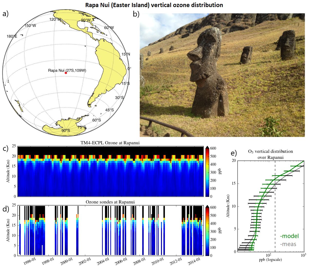
a) Easter Island map (a), ozone sonde data and back trajectories:Laura Gallardo, Adolfo HenrÍquez, Anne M. Thompson, Roberto Rondanelli, Jorge Carrasco, Andrea Orfanoz-Cheuquelaf & Patricio Velásquez (2016). The first twenty years (1994–2014) of ozone soundings from Rapa Nui (27°S, 109°W, 51 m a.s.l.), Tellus B: Chemical and Physical Meteorology, 68:1,DOI: 10.3402/tellusb.v68.29484

b) Moai picture (b): Matías Morel [CC BY-SA 4.0 (https://creativecommons.org/licenses/by-sa/4.0)], from Wikimedia Commons

c) Plots (c), (d) and (e): Dr. Nikos Daskalakis (IUP) from original data.

Modelling of the ozone vertical distribution

Introduction-Motivation: Modelling of ozone is a difficult task, since there are no direct ozone emissions. It is a purely secondary pollutant, chemically produced in the atmosphere. The main removal processes consist of chemical transformation and dry deposition. To simulate the vertical distribution of ozone in the troposphere, we need to properly account for both precursor species amounts (CO, NOx etc) and production/removal processes.

For this work, we used the highly documented TM4-ECPL model (Daskalakis et al., ACP, 2016 and references therein). TM4-ECPL is a Chemistry and Transport Model (CTM) with an analytical chemical scheme consisting of ~280 reactions involving 120 tracers (Myriokefalitakis et al., ACP, 2008, 2011). The model is driven by the ERA-Interim meteorology from ECMWF (Dee et al., GMD, 2011) and uses a variety of emissions covering all different sources (anthropogenic, biomass burning, biogenic, marine and soil).

Here we compare the simulated TM4-ECPL ozone concentrationsover the Easter Island (Rapa Nui) to the collocated time series of ozone sondes. Easter Island is chosen as a representative background site of the Southern Pacific region; making such a comparison extremely important for the understanding of the modeled processes. Such a remote location has minimal local anthropogenic impact on ozone precursor levels. This is supported by back trajectories of the region, which show that the air masses reaching the island come mainly from the west, being influenced mostly by the vast ocean (Gallardo et al., Tellus B, 2016).

The model-measurements comparison revealed that the model simulates correctly the seasonality of ozone levels. However, at the same time the comparison also pointed to model’s inability to simulate the tropopause height (panel (e)). The model simulates a higher tropopause affecting this way the mixing of the atmosphere. It manages to capture stratospheric ozone intrusions events that we see from the measurements with higher ozone values well below the tropopause, down to almost 10 km altitude (13 km altitude in the model). To further explain the ozone levels, the impact of long-range transport, wildfires and the El Niño-Southern Oscillation (ENSO) needs to be addressed.

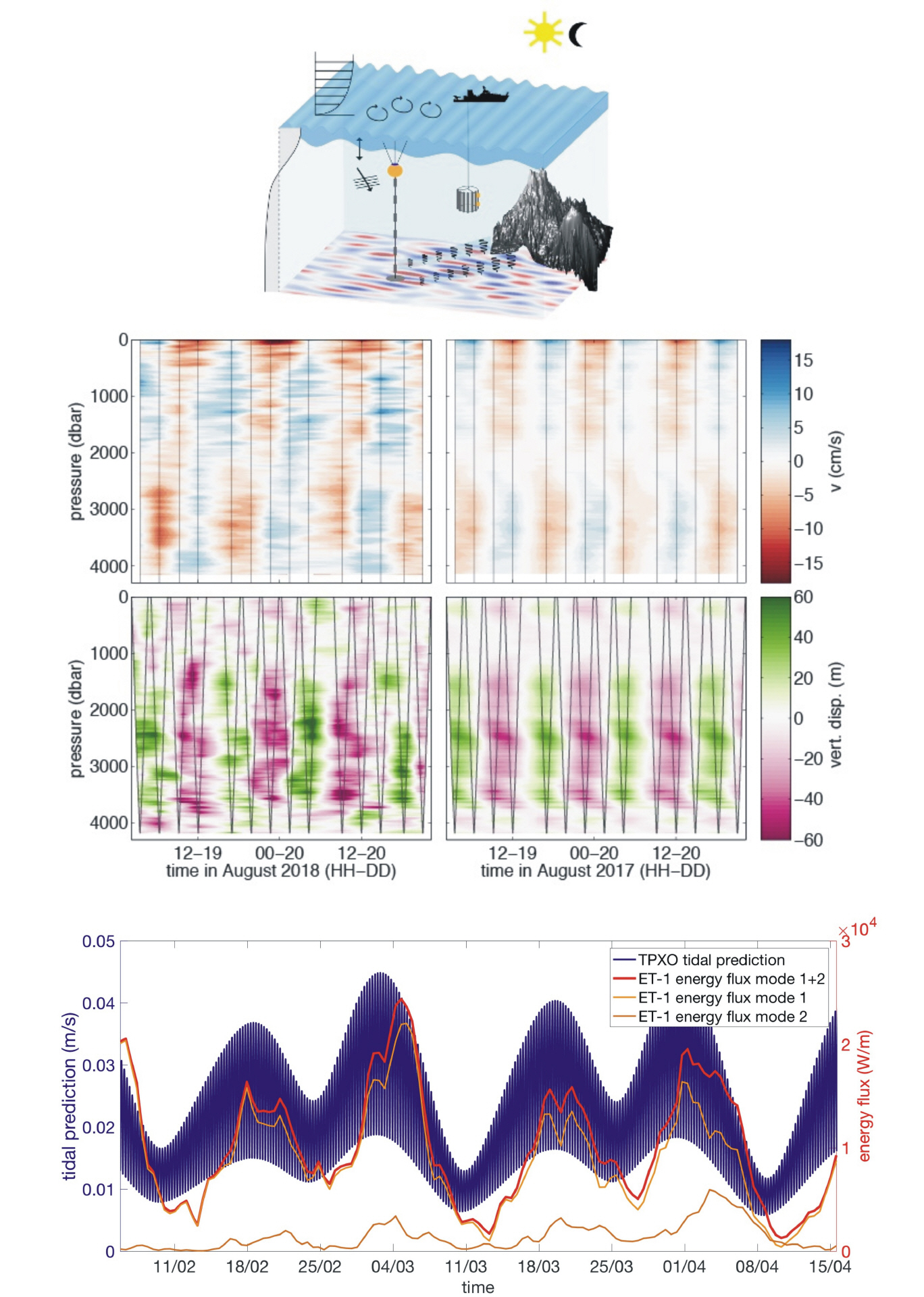
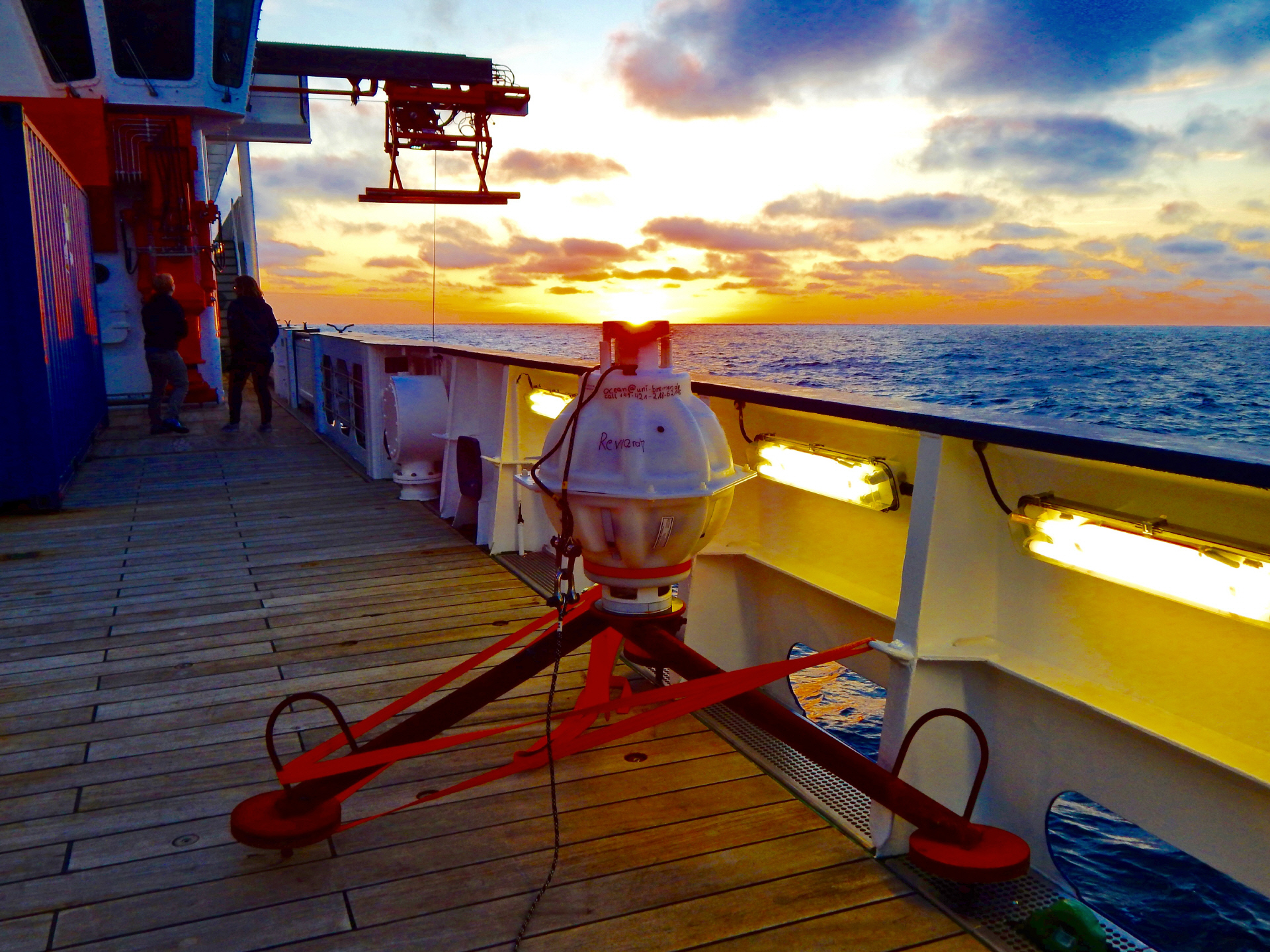
Internal wave energy fluxes in a tidal beam south of the Azores

Internal gravity waves in the ocean are generated by tides, wind, and interaction of currents with rough seafloor topography. Models predict a global energy supply for the internal wave field of about 0.7–1.3 TW by the conversion of barotropic tides at mid-ocean ridges and abrupt topographic features. Winds acting on the oceanic mixed layer contribute 0.3–1.5 TW and mesoscale flow over rough topography adds an additional amount of 0.2 TW. Globally, 1–2 TW are needed to maintain the observed stratification of the deep ocean by diapycnal mixing that results from the breaking of internal waves. Observations indicate that the energy available for mixing is redistributed by internal tides and near-inertial waves at low vertical wavenumber that can propagate thousands of kilometers from their source regions. While eddy-permitting global ocean circulation models are partly able to quantify the different sources of energy input and to simulate the propagation of the lowest internal wave modes, the variation and dissipation of the internal wave energy flux along its paths needs to be parameterized.

The figure shows results from an experiment south of the Azores, where a seamount chain is a major generation site of internal waves. The waves emanate from the seamounts a relatively narrow tidal beam, which makes the area an ideal observation site for the processes acting on the waves. The schematic shows the bathymetry of the seamounts on the right side, with the amplitude patternof the tidal beam as observed from satellite altimetry indicated in red and blue. Our instrumentation to observe the associated internal wave fluxes are the CTD/LADCP system below the ship (used for time series stations), and a long-term current meter/temperature logger mooring to observe temporal variability within the beam. The data shown are (bottom) an excerpt from the fluxes recorded by the mooring, decomposed into wave modes, and the corresponding predicted tidal velocity, and (top right) the internal wave signal in velocity (upper panel) and stratification (lower panel) observed during the time series stations, unfiltered (left), and filtered for the M2 internal tide (right) fluctuations.


Project:

TRR181 Energy Transfers in Atmosphere and Ocean (https://www.trr-energytransfers.de), Subproject W2: 'Energy transfer through low mode internal waves' Monika Rhein (MARUM/IUP, University of Bremen), Jin-Song von Storch (MPI for Meteorology, Hamburg) DFG

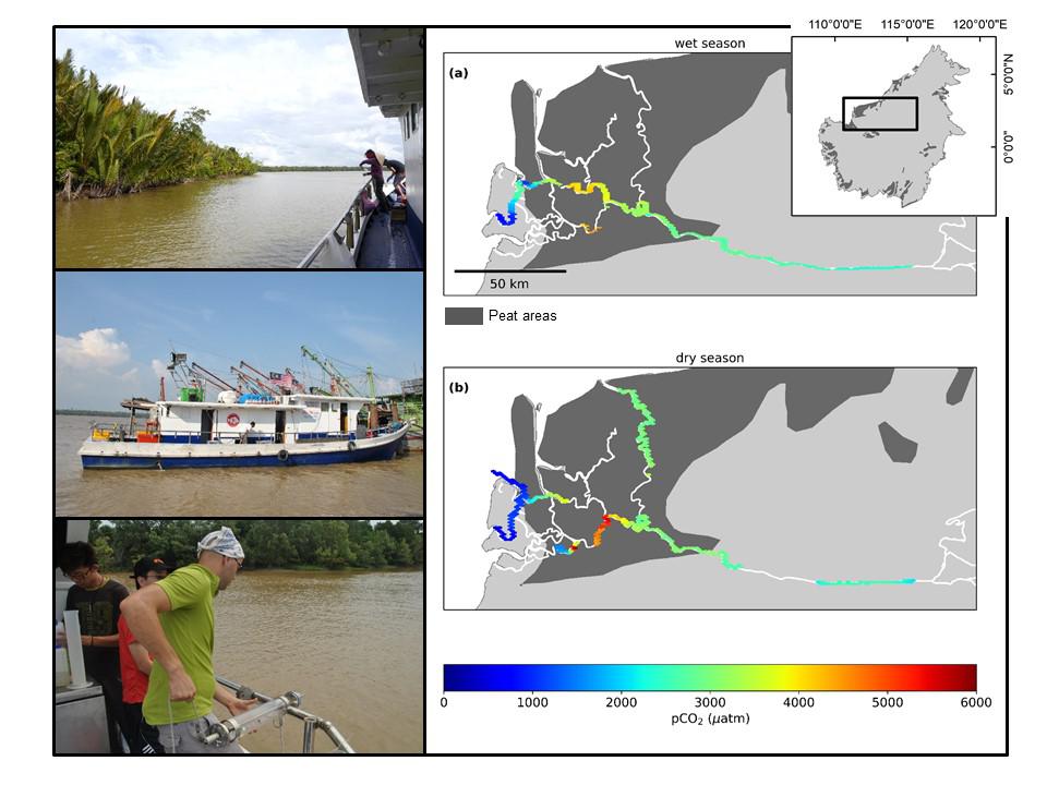
Carbon Dioxide Emissions from Southeast Asian Rivers

How much carbon dioxide (CO2) is released from Southeast Asian rivers? At the Institute of Environmental Physics (IUP), we have investigated this question in close collaboration with the Leibniz Center for Tropical Marine Research (ZMT), Bremen, and with the Swinburne University of Technology in Kuching, Malaysia. Our recent work, supported by the Central Development Research Fund of the University of Bremen, focused on the Rajang River, the longest river in Malaysia on the island of Borneo. It flows through mountainous terrain, tropical rainforests, oil palm plantations and peatlands. Southeast Asian peatlands store large amounts of organic carbon. It is expected that this carbon is released to the adjacent rivers, converted to CO2 and released to the atmosphere from the water surface. However, due to the proximity of the peatlands to the coast, the material is swiftly transported to the ocean, and CO2 emissions from Southeast Asian rivers are actually much lower than predicted. This was confirmed by our research at the Rajang River.

The left images are photographs of our scientists and students at work. The right image displays the measured partial pressure of CO2 (pCO2, in µatm) in the Rajang River. Peat areas are shown in dark colors. It can be seen that pCO2 increases as the river flows through the peat area, but soon decreases towards the river mouth due to mixing with seawater.

Our current knowledge of Southeast Asian river systems is mainly based on these kind of sampling campaigns. They can be realized in short term at relatively low cost and allow to resolve spatial patterns of carbon dynamics in a river. In order to better constrain the temporal variability of carbon fluxes in peat-draining rivers, it would be desirable to have additional long-term monitoring data. A new project, funded by the German Research Foundation (Deutsche Forschungsgemeinschaft, DFG), will look into the use of satellites to monitor the amount of riverine dissolved organic carbon (DOC), which is one of the most important drivers of CO2 emissions.

Related Projects:

‘Integrating field measurements and numerical modeling in order to understand carbon dynamics in Southeast Asian rivers’, awarded to Denise Müller-Dum (IUP), CDRF (Uni Bremen)
‘Studying dissolved organic carbon in tropical rivers of Malaysia using in-situ and satellite observations’, awarded to Justus Notholt (IUP), Thorsten Warneke (IUP), Tim Rixen (ZMT), DFG

Text and Images: Denise Müller-Dum (IUP) and Moritz Müller (Swinburne University of
Technology, Malaysia)

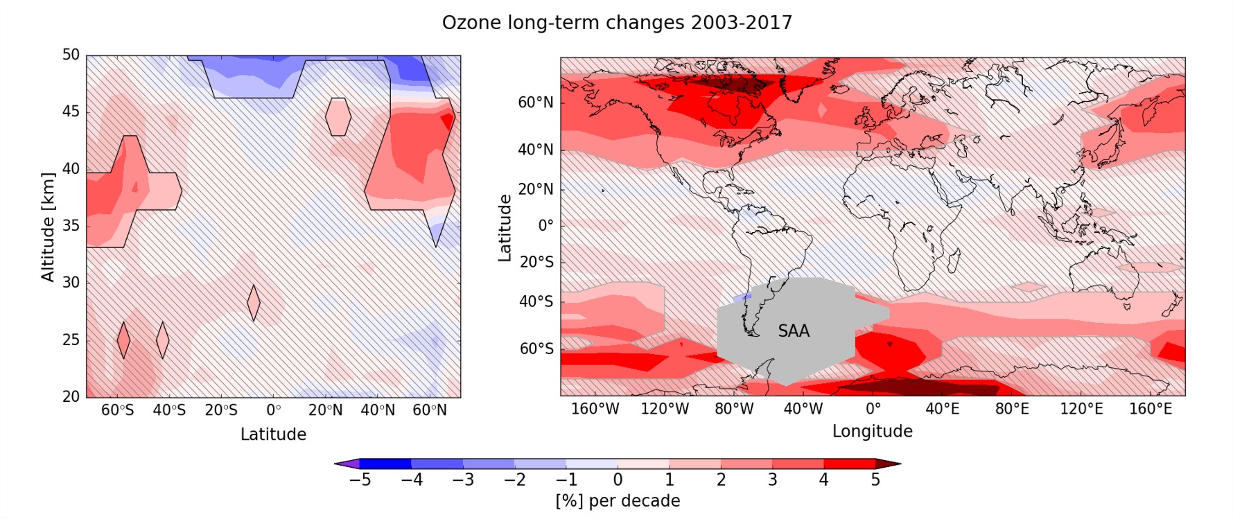
The left panel shows long-term changes in zonal monthly mean ozone in the stratosphere over the 2003-2017 period as a function of altitude and latitude. Values are reported in % per decade and shaded areas indicate non-significant trends. The right panel shows the longitudinally resolved long-term changes at an altitude of 38 km, displaying a remarkable variability. These plots confirm a significant increase of ozone concentration at mid latitudes in the upper stratosphere, whereas, in the middle stratosphere down to 20 km the long-term changesare generally not significant.

The observed increase of ozone concentration around 35-45 km is attributed by recent studies to two main causes; the first one is the decreasing concentration of ozone depleting substances after the production and use of CFCs have been regulated by the Montreal Protocol and its amendments. The second explanation is related to the increasing concentration of greenhouse gases responsible for the recorded global tropospheric warming. Due to radiative processes, this leads to a stratospheric cooling that in turn impacts on the ozone chemistry, increasing its production efficiency at these altitudes. Changes in the stratospheric circulation also have a strong influence on the latitudinal and vertical distribution of ozone and its trends.

In order to obtain a long term record of ozone profiles and study the long-term changes, SCIAMACHY and OMPS Limb Profiler stratospheric ozone data sets have been retrieved and merged at the University of Bremen. Since the overlap of the two satellite missions is only 3 months at the beginning of 2012, a reference time series for the merging has been used. Data from the NASA Aura-MLS instrument have been chosen for this purpose, as the instrument performs limb observations with a broad latitude coverage and it is considered stable and reliable.

Trends have been computed using a multilinear regression model, accounting for all phenomena having a strong impact on stratospheric ozone on different temporal and spatial scale: the solar activity, the quasi-biennial oscillation, El Nino and seasonal terms with a period of 6 and 12 months.

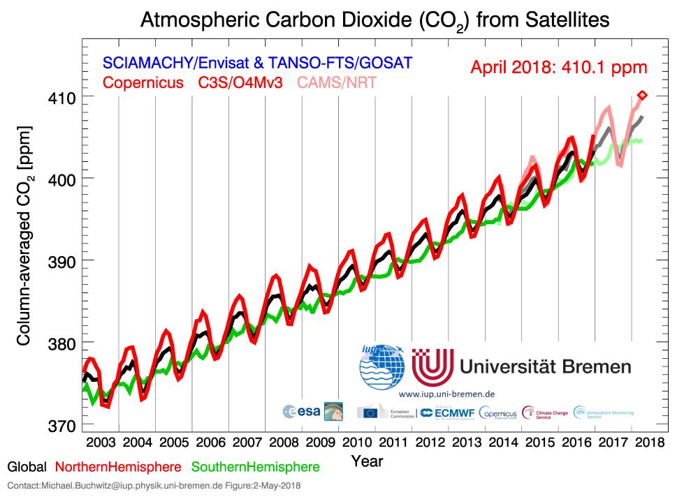
Atmospheric CO2 reaches new high-water mark

Satellite data show that northern hemispheric CO2 has exceeded 410 parts per million (ppm) in April 2018. Globally approximately 407.6 ppm has been reached. These are the highest atmospheric CO2concentrations since at least 800000 years.

The figure presents time series of atmospheric CO2 mixing ratios for the entire world (black and grey lines), for the northern hemisphere (red) and for the southern hemisphere (green). Shown are monthly mean column-averaged molecular mixing ratios of CO2 (“XCO2”) as retrieved from satellite measurements.

The lines shown in pale colours (recent years) correspond to preliminary time series generated in Near-Real-Time (NRT) whereas the bright colours show a high-quality Climate Data Record (CDR) currently covering the time period 2003-2016.

All curves show an increasing trend due to increasing concentrations of atmospheric CO2 originating primarily from the burning of fossil fuels (coal, oil, gas). The seasonal variations within each year are primarily due to uptake and release of CO2 by vegetation (photosynthesis, respiration, decay of organic matter). As can be seen, the largest variations are over the northern hemisphere (red line), where most of the terrestrial vegetation is located. The northern hemispheric CO2 maximum is typically reached in May. After that CO2concentrations will decrease because the growing plants will take up large amounts of CO2from the atmosphere.

The satellite-derived CO2 time series have been generated at the Institute of Environmental Physics (IUP) of the University of Bremen, Germany. They have been derived from spectroscopic measurements of the European satellite instrument SCIAMACHY on Envisat (2002-2012) and from TANSO-FTS onboard the Japanese GOSAT satellite (since 2009).

The underlying retrieval algorithms and corresponding CO2 data products have been generated in the framework of three European projects: the GHG-CCI project of ESA’s Climate Change Initiative and the EU projects Copernicus Climate Change Service (C3S) and Copernicus Atmosphere Monitoring Service (CAMS).

The CAMS data product (pale colours, recent years) is generated in quasi near-real-time at University of Bremen for the European Centre for Medium-Range Weather Forecasts (ECMWF) for CO2 forecasting and other applications within CAMS.

The bright colours show a Climate Data Record (2003-2016) generated at University of Bremen for C3S, which will be extended each year by one additional year. This data product is based on merging several high-quality data products generated in Europe (by University of Bremen, SRON and University of Leicester), in Japan (by the National Institute for Environmental Studies (NIES)) and in the USA (by NASA’s CO2 ACOS team). The merging algorithm has been developed at University of Bremen in order to generate a data product with the highest possible data quality for challenging carbon and climate applications.

The satellite CO2 observations are mean molecular mixing ratios (or mole fractions) of CO2 with respect to dry air averaged over the entire vertical extent of the atmosphere. 410 parts per million means that on average 1 million air molecules (excluding water vapour) contain 410 CO2 molecules in the air above a given location. Note that these column-averaged observations are similar but not identical to CO2 measurements at the surface carried out, for example, by NOAA.

Monitoring of the atmospheric CO2 concentration is important because increasing atmospheric concentrations lead to global warming as CO2 is an important greenhouse gas. Before the industrial revolution, the atmospheric concentration of CO2 was below approximately 280 ppm for at least the last 800000 years. Since then the amount of atmospheric CO2 has increased by more than 40%. The goal of the Paris Agreement on Climate Change is to reduce emissions of greenhouse gases to limit global warming to less than 2 degrees Celsius - or even better to less than 1.5 degrees - with respect to pre-industrial times. Achieving this goal requires a major international effort. It is currently unclear if this goal can be reached.

Text and Images: Michael Buchwitz, Maximilian Reuter, Stefan Noël

April 2018:

Further investigation on megacities: EMeRGe HALO campaign in East Asia

The measurement campaign of the project EMeRGe (Effect of Megacities on the Transport and Transformation of Pollutants on the Regional and Global Scales) in East Asia started in March 2018 and will continue till 09.04.2018.

EMeRGe (http://www.iup.uni-bremen.de/emerge/), led by the Institute of Environmental Physics of the University of Bremen,aims at improving the knowledge and prediction of the transport and transformation patterns of European and Asian pollutant outflows of megacities by using the HALO research aircraft (www.halo.dlr.de). The first measurement campaign in Europe was successfully carried out in summer 2017.

The HALO payload for EMeRGe combines in situ and remote sensing instruments measuring O3and aerosol precursors, aerosol amounts and composition. This information, which is gathered following optimal HALO transects and vertical profiling, enables the investigation of the photochemical evolution of the megacity plumes, the lifetime of the emissions and the transport of the air masses.

For the second EMeRGe campaign in East Asia, HALO left Germany on the 07.03 to reach its airbase in Tainan (Taiwan) where it will stay till the 7.04.2018. Around 140 flight hours will be flown to investigate the transport and transformation of emissions from the megacities Manila, Taipei, Seoul, Tokyo, Beijing, Shanghai and Guangzhou. Already 10 flights have been successfully performed in March 2018.

EMeRGe additionaly stimulates measurements and modelling studies within an international best effort research partnership with the European, Asian, and American science community. More than 50 partners from 16 different countries are participating in EMeRGe international. From them 27 are Asian partners. EMeRGe international facilitates a much more comprehensive integrated analysis of all sets of observational data products (i.e. aircraft, ground and satellite based data) in the study of the transport and transformation of plumes from MPCs.

Text and Images: Lola Andres Hernandez

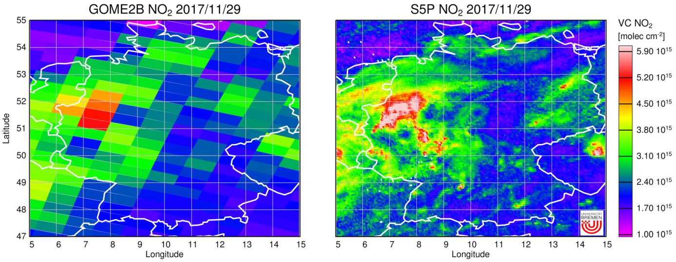
First NO2 results from the Sentinel-5 Precursor

On October 13, 2017, the Sentinel-5 precursor (S5P), the first of the atmospheric Copernicus instruments was successfully launched into an afternoon low earth orbit. The TROPOMI instrument on-board of this satellite continues the atmospheric remote sensing measurements of the GOME, SCIAMACHY, OMI and GOME-2 instruments. The main data products are O3, NO2, HCHO, CO, CH4 and cloud and aerosol information, but additional data products are possible and are currently being developed at several institutes, including IUP Bremen. Compared to previous instruments, S5P combines global coverage with excellent spatial resolution of 3.5 x 7 km2 (7 x 7 km2 in the SWIR), resulting in an unprecedented level of detail of the derived global maps.

The instrument is still in commissioning phase and official release of operational data is foreseen for July 2018. However, first spectra and lv2 products have already been made available to the core team and validation groups, and so far, data quality appears to be very good. Using the verification algorithms developed over the last years, IUP Bremen has used S5-P radiances and irradiances to produce first maps of CO, CH4, NO2, HCHO, H2O and BrO, all of which show good quality and interesting details.

As an example, data from one S5P overpass over Germany on November 29, 2017 is shown in the figure.


Disclaimer: The presented work has been performed within the framework of the Sentinel-5 Precursor Level 1/Level 2 Product Working Group activities. Results are based on preliminary (not fully calibrated/validated) Sentinel-5 Precursor data that are still subject to change.

Acknowledgement: Sentinel-5 Precursor is a European Space Agency (ESA) mission on behalf of the European Commission (EC). The TROPOMI payload is a joint development by ESA and the Netherlands Space Office (NSO). The Sentinel-5 Precursor ground-segment development has been funded by ESA and with national contributions from The Netherlands, Germany, and Belgium.

Links: http://www.tropomi.eu/

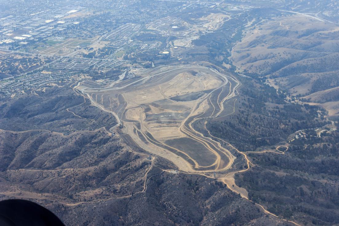
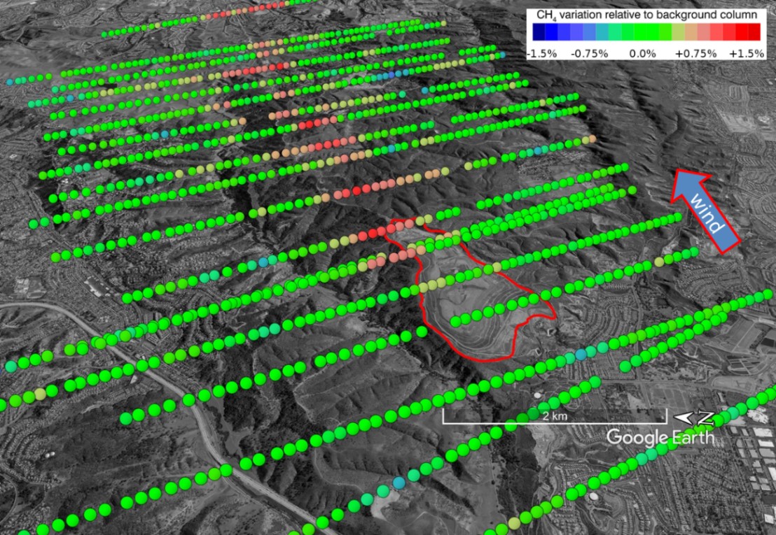
Methane emissions from Landfills

For the first time, scientists of the Institute of Environmental Physics successfully conducted an independent verification of total landfill methane emissions using airborne remote sensing techniques.

During a measurement campaign in California, methane concentrations around a landfill were measured using remote sensing techniques and a standard in-situ technique.

With the help of new sophisticated data analysis techniques and a comparison of the remote sensing data with data obtained from standard measurement technique, they were able to demonstrate that remotely sensed methane concentration data acquired from aircraft are accurate enough to verify reported methane emissions from a landfill. For the landfill under study, good agreement between reported and independently determined emission was found.

During the measurement campaign in California, methane emissions from oil fields were also measured (see also picture of the month April 2015 [LINK]). This research was highlighted in the TV magazine PlusMinus recently (December 2017).
Currently, the researchers are developing the next generation of airborne methane remote sensors, with a much better precision for methane detection of localized emitters.

Contact: heinrich.bovensmann@uni-bremen.de

Publication:

Krautwurst, S., Gerilowski, K., Jonsson, H. H., Thompson, D. R., Kolyer, R. W., Iraci, L. T., Thorpe, A. K., Horstjann, M., Eastwood, M., Leifer, I., Vigil, S. A., Krings, T., Borchardt, J., Buchwitz, M., Fladeland, M. M., Burrows, J. P., and Bovensmann, H.: Methane emissions from a Californian landfill, determined from airborne remote sensing and in situ measurements, Atmos. Meas. Tech., 10, 3429-3452, https://doi.org/10.5194/amt-10-3429-2017, 2017

Link: https://www.atmos-meas-tech.net/10/3429/2017/

TV magazine ARD PlusMinus from 7.12.2017

http://www.daserste.de/information/wirtschaft-boerse/plusminus/sendung/plusminus-erdgasfoerderung100.html

• Images of the month 2020 - 2021
• Images of the month 2018 - 2019
• Images of the month 2016 - 2017
• Images of the month 2014 - 2015